Preparing genomic data for phylogeny reconstruction
| Author(s) |
|
| Reviewers |
|
OverviewQuestions:
Objectives:
How do I find a set of common proteins (orthologs) across related species or strains?
How do I organize a set of orthologs to infer evolutionary relations between species or strains (phylogenetic reconstruction)?
Requirements:
Mask repetitive elements from a genome
Annotate (predict protein-coding genes) the genomes of the samples to compare
Find a set of common proteins across the samples (orthologs)
Align orthologs across samples
- Introduction to Galaxy Analyses
- slides Slides: An Introduction to Genome Assembly
- tutorial Hands-on: An Introduction to Genome Assembly
Time estimation: 3 hoursSupporting Materials:Published: Oct 21, 2022Last modification: Jun 3, 2025License: Tutorial Content is licensed under Creative Commons Attribution 4.0 International License. The GTN Framework is licensed under MITpurl PURL: https://gxy.io/GTN:T00132version Revision: 5
A robust and well-resolved phylogenetic classification is essential to understand genetic relationships within and between species and the evolution of their phenotypic diversity. In the last decade the genomic revolution has represented a drastic change in the amount of data used for phylogenetic inference. The single-gene approach using universal phylogenetic markers for the different lineages across the tree of life, is now being replaced by the assembly of taxon-rich and genome-scale data matrices, the so called phylogenomic approach.
Molecular sequence data can be used to construct a phylogeny by comparing differences between nucleotide or amino acid sequences across species or strains, a technique called phylogenomics. Young and Gillung 2019 have written a comprehensive review on the topic of phylogenomics.
In this tutorial we prepare genetic sequence data for phylogenetic reconstruction, using sequences from chromosome 5 of five strains of the yeast Saccharomyces cerevisiae.
To prepare the data, we will:
- Predict protein coding genes from the genome using Funannotate
- Find the proteins that are present in more than one genome, called orthologs, using Proteinortho and extract a subset with orthologs that are present in all samples.
- Align each set of orthologs using ClustalW.
The resulting dataset is ready to be used for phylogenetic reconstruction.
If you are starting from sequence reads, please follow An Introduction to Genome Assembly, and the appropriate genome assembly training for your sequencing technology from GTN’s Assembly section
AgendaIn this tutorial, we will cover:
Get data
For this training we will use a subset of the genome (chromosome 5) from four strains of S. cerevisiae. The GenBank annotated sequenced were produced using ‘funannotate predict annotation’ (Galaxy Version 1.8.9+galaxy2) on the nucleotide sequences sequences.
Hands On: Data upload
- Create a new history for this tutorial
Import the files from Zenodo or from the shared data library (
GTN - Material->ecology->Preparing genomic data for phylogeny reconstruction):https://zenodo.org/record/6610704/files/BK006939.2.genbank https://zenodo.org/record/6610704/files/BK006939.2.genome.fasta https://zenodo.org/record/6610704/files/CM000925.1.genbank https://zenodo.org/record/6610704/files/CM000925.1.genome.fasta https://zenodo.org/record/6610704/files/CM005043.2.genbank https://zenodo.org/record/6610704/files/CM005043.2.genome.fasta https://zenodo.org/record/6610704/files/CM005299.1.genbank https://zenodo.org/record/6610704/files/CM005299.1.genome.fasta
- Copy the link location
Click galaxy-upload Upload at the top of the activity panel
- Select galaxy-wf-edit Paste/Fetch Data
Paste the link(s) into the text field
Press Start
- Close the window
- Optional: Rename each dataset to its accession number followed by ‘.genome.fasta’ or ‘.genbank’.
Group the datasets into collections. These will ease data handling and help minimize the clutter in your history. Make a collection of nucleotide sequences and another of protein sequences.
- Click on galaxy-selector Select Items at the top of the history panel
- Check all the datasets in your history you would like to include
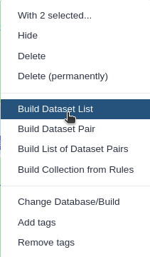
Click n of N selected and choose Advanced Build List
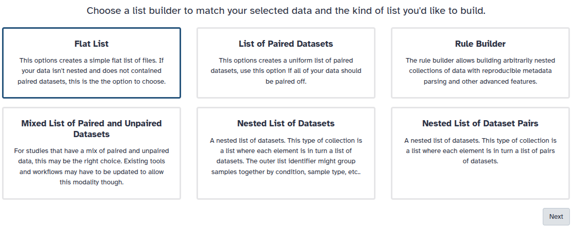
You are in collection building wizard. Choose Flat List and click ‘Next’ button at the right bottom corner.
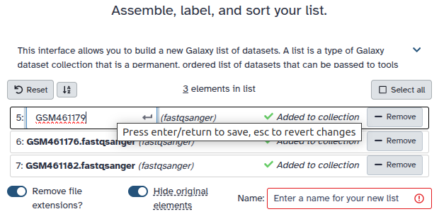
Double clcik on the file names to edit. For example, remove file extensions or common prefix/suffixes to cleanup the names.
- Enter a name for your collection
- Click Build to build your collection
- Click on the checkmark icon at the top of your history again


Protein coding gene prediction
Mask repetitive sequences
Before we can annotate the genome, we will prepare the data by masking repetitive sequences in the genome. Repeat-rich regions can interfere with genome annotation tools. In this step we find and soft-mask repetitive regions in the genome. The annotation tool can then take this information into account (see RepeatMasker tutorial for more details). We use RepeatMasker Smit et al. 2013, a program that screens DNA sequences for interspersed repeats and low complexity DNA sequences. This program has historically made use of RepBase (Kohany et al. 2006), a service of the Genetic Information Research Institute, but this database in no longer open access. Instead, we will use Dfam (Storer et al. 2021) an open collection of Transposable Element DNA sequence alignments, HMMs derived from Repbase sequences and consensus sequences. For this reason, the annotation of repetitive sequences might be incomplete.
RepeatMasker will only accept compact fasta headers. Before we can mask repetitive regions with RepeatMasker we must trim the NCBI long header (BK006939.2 TPA_inf: Saccharomyces cerevisiae S288C chromosome V, complete sequence) to leave only the accession number (>BK006939.2) by using a regular expression.
Hands On: Mask repetitive sequences
- Replace Text ( Galaxy version 1.1.2) with the following parameters:
- param-collection “File to process”:
output(Input dataset collection)- In “Replacement”:
- param-repeat “Insert Replacement”
- “Find pattern”:
(>[^ ]+).+“Replace with:”:
\1Comment
\1replaces the text in the header with the first matched text in the header, the accession number in this case.- RepeatMasker ( Galaxy version 4.1.2-p1+galaxy0) with the following parameters:
- param-file “Genomic DNA”:
outfile(output of Replace Text tool)- “Repeat library source”:
DFam (curated only, bundled with RepeatMasker)
- “Select species name from a list?”:
No
- “Repeat source species”:
"Saccharomyces cerevisiae"CommentIf you don’t select the species from the list, you must provide a species name (“Saccharomyces cerevisiae” in this example). In principal, all unique clade names occurring in NCBI taxonomy database can be used for species. Capitalization is ignored, multiple words need to bound by apostrophes. Not all “common” English names occur in the taxonomy database. Using Latin names is always safest.
- Inspect the ‘RepeatMasker masked sequence on data’ output file. Scroll down and you will find stretches of ‘N’ on the location of repetitive sequences. The file is now ready for annotation with Funannotate.
Annotate with Funannotate
We will predict protein-coding genes from genomic sequences using Funannotate (Young and Gillung 2019), which collects evidence from different ab-initio gene predictors as well as from RNA-seq or ESTs data. Funannotate has been developed for Fungi but it works with any Eukaryotic genome. The output of Funannotate is a list of ORFs and their translation in GenBank format.
CommentIf you would like to learn about genome annotation in more depth, the GTN has a section dedicated to training on genome annotation, including a hands-on tutorial on Funannotate.
Warning: Slow Step Ahead!Even for a small dataset, Funannotate can take a very long time to run. You can skip this step and use the Genbank files downloaded from Zenodo for the following step. These were generated using Funannotate as described in the hands-on below.
Hands On: Annotate genome
- Funannotate predict annotation ( Galaxy version 1.8.9+galaxy2) with the following parameters:
- param-file “Assembly to annotate”:
output_masked_genome(output of RepeatMasker tool)- In “Organism”:
- “Name of the species to annotate”:
Saccharomyces cerevisiae- “Is it a fungus species?”:
Yes- “Ploidy of assembly”:
1- In “Evidences”:
- “Select protein evidences”:
Use UniProtKb/SwissProt (from selected Funannotate database)If available, include mRNA and/or ESTs in this evidence section to increase sensitivity of predictions.
- In “Busco”:
- “BUSCO models to align”:
saccharomycetes- “Initial Augustus species training set for BUSCO alignment”:
saccharomyces- In “Augustus settings (advanced)”:
- “Minimum number of models to train Augustus”:
15CommentWhen annotating full genomes, increase the number of ‘Minimum number of models to train Augustus’ to an appropriate value. For the small sample dataset used here, values larger than 15 will result in failure.
- Inspect the output GenBank file. The FEATURES section contains the genome annotation of protein predictions, their location and their translation. Each predicted protein is given a unique ID, which will become the FASTA header in the next step.
Extract ORFs into FASTA files
In this step, we extract the protein sequences from the GenBank files into multi-FASTA files. Additionally, we modify the headers to include the accession number of the sample. This creates an unique accession-proteinID header for each predicted protein, and will allow us to retrieve them after we combine all predicted proteins into one multi-FASTA file.
So far, we have kept sequence files in a collection. Now we will combine all predicted proteins from all samples into one big multi-fasta file. Later, we will retrieve ortholog sequences from this file.
Hands On: Extract ORFs
- Extract ORF ( Galaxy version 3.02) with the following parameters:
- param-file “gene bank file”:
annot_gbk(output of Funannotate predict annotation tool - or the genbank files downloaded from Zenodo)- Regex Find And Replace ( Galaxy version 1.0.1) with the following parameters:
- param-file “Select lines from”:
aa_output(output of Extract ORF tool)- In “Check”:
- param-repeat “Insert Check”
- “Find Regex”:
>([^ ]+).+- “Replacement”:
>#{input_name}_\1- Collapse Collection ( Galaxy version 4.2) with the following parameters:
- param-file “Collection of files to collapse into single dataset”:
out_file1(output of Regex Find And Replace tool)- “Prepend File name”:
Yes
Question
- Is the number of predicted ORFs the same across the samples?
- No, the number of predicted ORFs ranges from 193 to 199.
Find orthologs
Orthologs are genes in different species evolved from a common ancestral gene by a speciation (lineage-splitting) event and contain the information needed for building phylogenies. The input for this step is the collection of multi-FASTA extracted from the GenBank file and modified to have unique headers. The result file ‘orthology-groups’ contains one row per orthogroup and one column per sample.
Next, we select orthogroups where all the species are represented by only one protein, 1:1 single copy orthologs (a total of 4 proteins per orthogroup for this dataset).
Hands On: Find and filter orthologs
- Proteinortho ( Galaxy version 6.0.14+galaxy2.9.1) with the following parameters:
- param-file “Select the input fasta files (>2)”:
out_file1(output of Regex Find And Replace tool)- “Activate synteny feature (POFF)”:
no- Filter with the following parameters:
- param-file “Filter”:
proteinortho(output of Proteinortho tool)- “With following condition”:
c1==4 and c2==4- Inspect the ‘orthology-groups’ tabular file.
Question
Inspect the the ‘orthology-groups’ tabular file.
- Do any samples contain more than one gene for any given orthogroup?
- What is the name given to these homologous genes within the same genome?
- Yes, CM000925.1 contains two genes on the first orthogroup.
- Paralogs. These are gene copies created by a duplication event within the same genome.
Look at the filtered orthogroups.
- How many orthogroups are represented once only in all four samples?
- 173
Quality control with Busco
Busco is a dataset of nearl-universal, single-copy orthologs. Here we use it for quality control of the assembly and annotation produced above. It outputs a proxy of completeness, duplication and fragmentation of the annotation (Busco can also be used to assess the completeness of a genome assembly).
Hands On: QC with Busco
- Busco ( Galaxy version 4.1.4) with the following parameters:
- param-file “Sequences to analyse”:
out_file1(output of Regex Find And Replace tool)- “Mode”:
Proteome- “Lineage”:
Saccharomycetes- In “Advanced Options”:
- “Augustus species model”:
Use the default species for selected lineageMake sure you select the ‘lineage’ closest to the species(s) you are analyzing.
Question
- The Complete (‘C’) metric stands for complete Busco genes identified. Look at the Busco output file ‘Short summary’ for sample BK006939.2. What is the ‘C’ number?
- Why is it so low?
- 4.0%
- Our dataset contains only chromosome 5 of the yeast genome.
Extract proteins with Proteinortho
Next we extract 1:1 single copy orthologs and generate one multi fasta file per ortholog.
Hands On: Extract protein sequences
- Proteinortho grab proteins ( Galaxy version 6.0.14+galaxy2.9.1) with the following parameters:
- param-file “Select the input fasta files”:
output(output of Collapse Collection tool)- “Query type”:
orthology-groups output file
- param-file “A orthology-groups file”:
out_file1(output of Filter tool)
The output is a collection of multi-fasta ortholog files. All species are represented in each file and are ready to be aligned.
Align ortholog sequences
Alignment of sequences allows cross-species (or other taxonomic level, strain, taxa) comparison. An alignment is a hypothesis of positional homology between bases/amino acids of different sequences. A correct alignment is crucial for phylogenetic inference. Here we use ClustaW, a well-established pairwise sequence aligner.
First we modify the headers of the multi-fasta file, such that only the sample name is retained. This is important for future conatenation of alignment into a supermatrix (see Maximum likelihood GTN training)
Hands On: Align orthologs with ClustalW
- Regex Find And Replace ( Galaxy version 1.0.1) with the following parameters:
- param-file “Select lines from”:
listproteinorthograbproteins(output of Proteinortho grab proteins tool)- In “Check”:
- param-repeat “Insert Check”
- “Find Regex”:
(>[^_]+).+- “Replacement”:
\1- ClustalW ( Galaxy version 2.1) with the following parameters:
- param-file “FASTA file”:
out_file1(output of Regex Find And Replace tool)- “Data type”:
Protein sequences- “Output alignment format”:
FASTA format- “Output complete alignment (or specify part to output)”:
Complete alignment
Question
- Open the ClustalW output ‘queryOrthoGroup121.fasta’ and its corresponding multifasta input. You can compare them side by side activating the ‘Scratchbook’ on the top panel. What is the main difference between the sequences in the unaligned multifasta (input) and the ClustalW output multifasta?
- Two of the sequences from this orthogroup are truncated (early stop codon). The alignment program inserts ‘-‘ to represent indels in the alignment.
Conclusion
In this tutorial, you have prepared genome sequence data for phylogenetic analysis. First, you have extracted information from these in the form of predicted protein sequences. You then grouped the predicted proteins into orthogroups and aligned them. These aligned sequences can now be used for reconstructing a phylogeny and building a phylogenetic tree.
You've Finished the Tutorial
Key points
You now are able to
Predict proteins in a nucleotide sequence de-novo using funannotate_predict
Find orthologs across different samples with orthofinder
Align orthologs with ClustalW in preparation for phylogeny reconstruction
Frequently Asked Questions
Have questions about this tutorial? Have a look at the available FAQ pages and support channelsUseful literature
Further information, including links to documentation and original publications, regarding the tools, analysis techniques and the interpretation of results described in this tutorial can be found here.
References
- Kohany, O., A. J. Gentles, L. Hankus, and J. Jurka, 2006 Annotation, submission and screening of repetitive elements in Repbase: RepbaseSubmitter and Censor. BMC Bioinformatics 7: 474.
- Smit, A. F. A., R. Hubley, and P. Green, 2013 RepeatMasker Open-4.0.
- Young, A. D., and J. P. Gillung, 2019 Phylogenomics — principles, opportunities and pitfalls of big-data phylogenetics. Systematic Entomology 45: 225–247. 10.1111/syen.12406
- Storer, J., R. Hubley, J. Rosen, T. J. Wheeler, and A. F. Smit, 2021 The Dfam community resource of transposable element families, sequence models, and genome annotations. Mobile DNA 12: 10.1186/s13100-020-00230-y
Feedback
Did you use this material as an instructor? Feel free to give us feedback on how it went.
Did you use this material as a learner or student? Click the form below to leave feedback.

Citing this Tutorial
- Miguel Roncoroni, Brigida Gallone, Preparing genomic data for phylogeny reconstruction (Galaxy Training Materials). https://training.galaxyproject.org/training-material/topics/ecology/tutorials/phylogeny-data-prep/tutorial.html Online; accessed TODAY
- Hiltemann, Saskia, Rasche, Helena et al., 2023 Galaxy Training: A Powerful Framework for Teaching! PLOS Computational Biology 10.1371/journal.pcbi.1010752
- Batut et al., 2018 Community-Driven Data Analysis Training for Biology Cell Systems 10.1016/j.cels.2018.05.012
Congratulations on successfully completing this tutorial!@misc{ecology-phylogeny-data-prep, author = "Miguel Roncoroni and Brigida Gallone", title = "Preparing genomic data for phylogeny reconstruction (Galaxy Training Materials)", year = "", month = "", day = "", url = "\url{https://training.galaxyproject.org/training-material/topics/ecology/tutorials/phylogeny-data-prep/tutorial.html}", note = "[Online; accessed TODAY]" } @article{Hiltemann_2023, doi = {10.1371/journal.pcbi.1010752}, url = {https://doi.org/10.1371%2Fjournal.pcbi.1010752}, year = 2023, month = {jan}, publisher = {Public Library of Science ({PLoS})}, volume = {19}, number = {1}, pages = {e1010752}, author = {Saskia Hiltemann and Helena Rasche and Simon Gladman and Hans-Rudolf Hotz and Delphine Larivi{\`{e}}re and Daniel Blankenberg and Pratik D. Jagtap and Thomas Wollmann and Anthony Bretaudeau and Nadia Gou{\'{e}} and Timothy J. Griffin and Coline Royaux and Yvan Le Bras and Subina Mehta and Anna Syme and Frederik Coppens and Bert Droesbeke and Nicola Soranzo and Wendi Bacon and Fotis Psomopoulos and Crist{\'{o}}bal Gallardo-Alba and John Davis and Melanie Christine Föll and Matthias Fahrner and Maria A. Doyle and Beatriz Serrano-Solano and Anne Claire Fouilloux and Peter van Heusden and Wolfgang Maier and Dave Clements and Florian Heyl and Björn Grüning and B{\'{e}}r{\'{e}}nice Batut and}, editor = {Francis Ouellette}, title = {Galaxy Training: A powerful framework for teaching!}, journal = {PLoS Comput Biol} }
You can use Ephemeris's
shed-tools installcommand to install the tools used in this tutorial.shed-tools install [-g GALAXY] [-a API_KEY] -t <(curl https://training.galaxyproject.org/training-material/api/topics/ecology/tutorials/phylogeny-data-prep/tutorial.json | jq .admin_install_yaml -r)Alternatively you can copy and paste the following YAML
---
install_tool_dependencies: true
install_repository_dependencies: true
install_resolver_dependencies: true
tools:
- name: glimmer_gbk_to_orf
  owner: bgruening
  revisions: '04861c9bbf45'
  tool_panel_section_label: Annotation
  tool_shed_url: https://toolshed.g2.bx.psu.edu/
- name: repeat_masker
  owner: bgruening
  revisions: 39b40a9a6296
  tool_panel_section_label: Annotation
  tool_shed_url: https://toolshed.g2.bx.psu.edu/
- name: text_processing
  owner: bgruening
  revisions: d698c222f354
  tool_panel_section_label: Text Manipulation
  tool_shed_url: https://toolshed.g2.bx.psu.edu/
- name: clustalw
  owner: devteam
  revisions: d6694932c5e0
  tool_panel_section_label: Multiple Alignments
  tool_shed_url: https://toolshed.g2.bx.psu.edu/
- name: regex_find_replace
  owner: galaxyp
  revisions: ae8c4b2488e7
  tool_panel_section_label: Text Manipulation
  tool_shed_url: https://toolshed.g2.bx.psu.edu/
- name: busco
  owner: iuc
  revisions: 602fb8e63aa7
  tool_panel_section_label: Annotation
  tool_shed_url: https://toolshed.g2.bx.psu.edu/
- name: funannotate_predict
  owner: iuc
  revisions: 2bba2ff070d9
  tool_panel_section_label: Annotation
  tool_shed_url: https://toolshed.g2.bx.psu.edu/
- name: proteinortho
  owner: iuc
  revisions: 4850f0d15f01
  tool_panel_section_label: Proteomics
  tool_shed_url: https://toolshed.g2.bx.psu.edu/
- name: collapse_collections
  owner: nml
  revisions: 830961c48e42
  tool_panel_section_label: Collection Operations
  tool_shed_url: https://toolshed.g2.bx.psu.edu/
- name: clipkit
  owner: padge
  revisions: '770695339600'
  tool_panel_section_label: Phylogenetics
  tool_shed_url: https://toolshed.g2.bx.psu.edu/
- name: phykit
  owner: padge
  revisions: 1ac6ee298657
  tool_panel_section_label: Evolution
  tool_shed_url: https://toolshed.g2.bx.psu.edu/