Genome assembly with Velvet: Background

Velvet is one of a number of de novo assemblers that use short read sets as input (e.g. Illumina Reads). The assembly method is based on the manipulation of de Bruijn graphs, via the removal of errors and the simplification of repeated regions.

Comment

For information about Velvet, you can check its (nice) Wikipedia page.

For this tutorial, we have a set of reads from an imaginary Staphylococcus aureus bacterium with a miniature genome (197,394 bp). Our mutant strain read set was sequenced with the whole genome shotgun method, using an Illumina DNA sequencing instrument. From these reads, we would like to rebuild our imaginary Staphylococcus aureus bacterium via a de novo assembly of a short read set using the Velvet assembler.

We also have a sequence for a reference genome that we will use later in the tutorial.

Agenda

In this tutorial, we will deal with:

1. Genome assembly with Velvet: Background
2. Get the data
3. Evaluate the input reads
4. Assemble reads with Velvet
5. Collect some statistics on the contigs
6. Discussion

Get the data

Hands-on: Getting the data

1. Create and name a new history for this tutorial.

   Tip: Creating a new history

   To create a new history simply click the new-history icon at the top of the history panel:

   

2. Import from Zenodo or from the data library the files:

   https://zenodo.org/record/582600/files/mutant_R1.fastq
   https://zenodo.org/record/582600/files/mutant_R2.fastq
   https://zenodo.org/record/582600/files/wildtype.fna
   

   Tip: Importing data via links

   • Copy the link location (Right-click on the filename then “Copy Link Address”)
   • Open the Galaxy Upload Manager
   • Select Paste/Fetch Data
   • Paste the link into the text field
   • For the read files, change the data-type to fastqsanger
   • Press Start

3. Change the name of the files to mutant_R1, mutant_R2 and wildtype.fna.

   As a default, Galaxy uses the link as the name of the new dataset. It also does not link the dataset to a database or a reference genome.

   Tip: Renaming a dataset

   • Click on the galaxy-pencil pencil icon for the dataset to edit its attributes
   • In the central panel, change the Name field
   • Click the Save button

4. Inspect the content of a file.

   Tip: Inspecting the content of a dataset

   • Click on the galaxy-eye (eye) icon next to the relevant history entry
   • View the content of the file in the central panel

   Question

   1. What are four key features of a FASTQ file?
   2. What is the main difference between a FASTQ and a FASTA file?

   Solution

   1. Each sequence in a FASTQ file is represented by 4 lines: 1st line is the id, 2nd line is the sequence, 3rd line is not used, and 4th line is the quality of sequencing per nucleotide
   2. In a FASTQ file, not only are the sequences present, but information about the quality of sequencing is also included.

The reads have been sequenced from an imaginary Staphylococcus aureus bacterium using an Illumina DNA sequencing instrument. We obtained the 2 files we imported (mutant_R1 and mutant_R2)

Question

Why do we have 2 files here if we only sequenced the bacteria once?

Solution

1. The bacteria has been sequenced using paired-end sequencing. The first file corresponds to forward reads and the second file to reverse reads.

Evaluate the input reads

Before doing any assembly, the first questions you should ask about your input reads include:

• What is the coverage of my genome?
• How good is my read set?
• Do I need to ask for a new sequencing run?
• Is it suitable for the analysis I need to do?

We will evaluate the input reads using the FastQC tool. This tool runs a standard series of tests on your read set and returns a relatively easy-to-interpret report. We will use it to evaluate the quality of our FASTQ files and combine the results with MultiQC.

Hands-on: FastQC on a fastq file

1. FastQC ( Galaxy version 0.73+galaxy0) with the following parameters:
   • param-files “Raw read data from your current history”: mutant_R1.fastq and mutant_R2.fastq

   Tip: Select multiple datasets

   1. Click on param-files Multiple datasets
   2. Select several files by keeping the Ctrl (or COMMAND) key pressed and clicking on the files of interest

2. MultiQC ( Galaxy version 1.11+galaxy1) with the following parameters:
   • “Results: Which tool was used to generate logs?”: FastQC
   • Click “Insert FastQC output”
   • “Type of FastQC output?”: multiple datasets, select the raw data files from FastQC

MultiQC generates a webpage combining reports for FastQC on both datasets. It includes these graphs and tables:

• General statistics

  We need to know about the data for our analysis. In particular, we need to know the read lengths as it is important in setting the maximum k-mer size for an assembly.

  Comment: Getting the length of sequences

  • Find the MultiQC output that is a webpage and click to view
  • The first table shows General Statistics for the input read files
  • At the top of this table, click on Configure Columns
  • Make sure the box next to Length is ticked
  • Close the window
  • This table should now show a column for read lengths

  Question

  1. How long are the sequences?
  2. What is the average coverage of the genome, given our imaginary Staphylococcus aureus bacterium has a genome of 197,394 bp?

  Solution

  1. The sequences are 150 bp long
  2. We have 2 x 12,480 sequences of 150 bp, so the average genome coverage is: 2 * 12480 * 150 / 197394, or approximately 19 X coverage.

• Sequence Quality Histograms

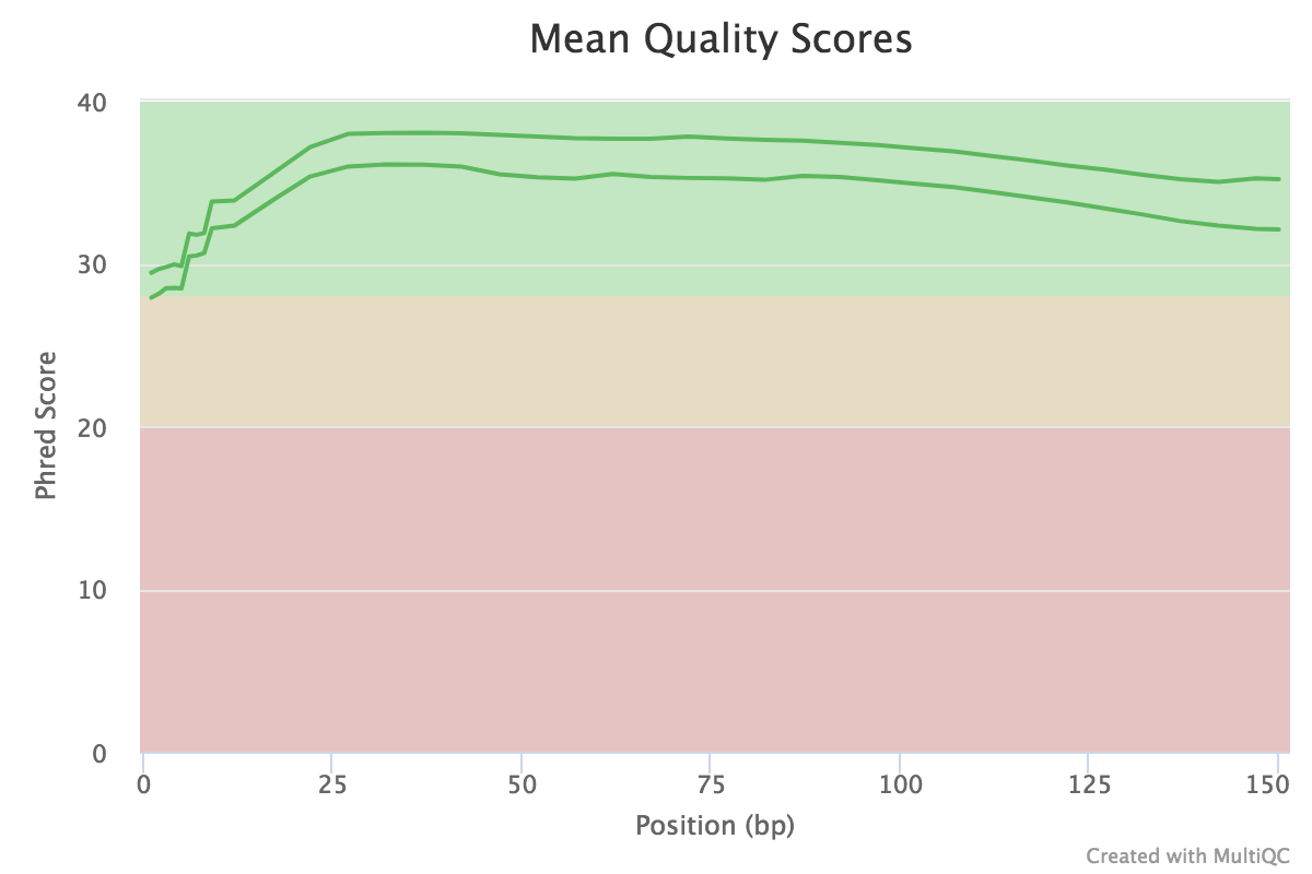
  Dips in quality near the beginning, middle or end of the reads may determine the trimming/cleanup methods and parameters to be used, or may indicate technical problems with the sequencing process/machine run.

  Open image in new tab
  
  

  Question

  1. What does the y-axis represent?
  2. Why is the quality score decreasing across the length of the reads?

  Solution

  1. The y-axis represents the quality score for each base (an estimate of the error during sequencing).
  2. The quality score is decreasing accross the length of the reads because the sequencing become less and less reliable at the end of the reads.

• Per Sequence GC Content

  High GC organisms tend not to assemble well and may have an uneven read coverage distribution.

• Per Base N Content

  The presence of large numbers of Ns in reads may point to a poor quality sequencing run. You will need to trim these reads to remove Ns.

• k-mer content

  The presence of highly recurring k-mers may point to contamination of reads with barcodes or adapter sequences.

Comment

For a fuller discussion of FastQC outputs and warnings, see the FastQC website link, including the section on each of the output reports, and examples of “good” and “bad” Illumina data.

We won’t be doing anything to these data to clean it up as there isn’t much need. Therefore we will get on with the assembly!

Assemble reads with Velvet

Now, we want to assemble our reads to find the sequence of our imaginary Staphylococcus aureus bacterium. We will perform a de novo assembly of the reads into long contiguous sequences using the Velvet short read assembler.

The first step of the assembler is to build a de Bruijn graph. For that, it will break our reads into k-mers, i.e. fragments of length k. Velvet requires the user to input a value of k (k-mer size) for the assembly process. Small k-mers will give greater connectivity, but large k-mers will give better specificity.

Hands-on: Assemble the reads

1. FASTQ interlacer ( Galaxy version 1.2.0.1+galaxy0) with the following parameters:
   • “Type of paired-end datasets”: 2 separate datasets
   • “Left-hand mates”: mutant_R1.fastq
   • “Right-hand mates”: mutant_R2.fastq

   Currently our paired-end reads are in 2 files (one with the forward reads and one with the reverse reads), but Velvet requires only one file, where each read is next to its mate read. In other words, if the reads are indexed from 0, then reads 0 and 1 are paired, 2 and 3, 4 and 5, etc. Before doing the assembly per se, we need to prepare the files by combining them.

2. velveth ( Galaxy version 1.2.10.3) with the following parameters:
   • “Hash Length”: 29
   • “Input Files”
     • Click on param-repeat “Input Files”
     • In “1: Input Files”
       • “Choose the input type”: interleaved paired end
       • “read type”: shortPaired reads
       • param-files “Dataset”: pairs output of FASTQ interlacer

   The tool takes our reads and break them into k-mers.

3. velvetg ( Galaxy version 1.2.10.2) with the following parameters:
   • param-files “Velvet Dataset”: outputs of velveth
   • “Using Paired Reads”: Yes

   This last tool actually does the assembly.

Five files are generated. We will look at the contigs file and the stats file:

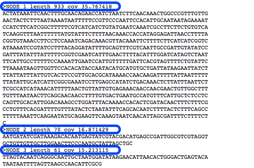
• The Contigs file

  This file contains the sequences of the contigs. In the header of each contig, a bit of information is added:

  • the k-mer length (called “length”): For the value of k chosen in the assembly, a measure of how many k-mers overlap (by 1 bp each overlap) to give this length
  • the k-mer coverage (called “coverage”): For the value of k chosen in the assembly, a measure of how many k-mers overlap each base position (in the assembly).
  • Note that your results may look different to the example in the image below.

  

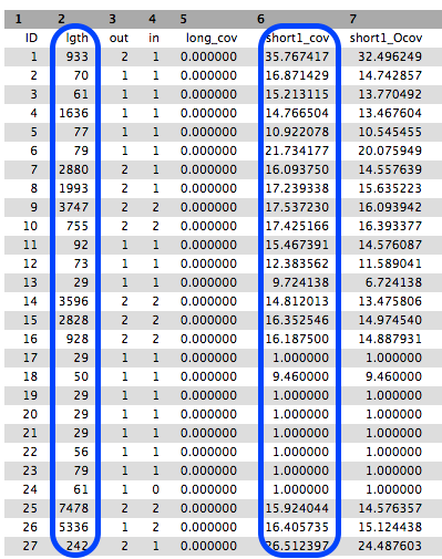
• The Stats file

  This is a tabular file giving for each contig the k-mer lengths, k-mer coverages and other measures. Note that your results may look different to the example in the image below.

  

Collect some statistics on the contigs

Question

1. How many contigs have been built?
2. What is the mean, min and max length of the contigs?

Solution

1. 306
2. To compute this information, we can use the Datamash tool on the 2nd columns (length). Be careful with the first line, the header. As a result, we obtain approximately: 516 as mean, 1 as min and 8836 as max. It would mean that the smallest contig has a length of 1 bp, even smaller than k. The length on the 2nd column corresponds to length of the contig in k-mers. This means that the smallest contig has a length of 1k = 29. So to obtain the real length, we need to add k-1 to the length. We then obtain a mean contig length of 544 bp, a min contig of 29 bp and a max contig of 8864 bp.

This table is limitted, but we will now collect more basic statistics on our assembly.

Hands-on: Collect fasta statistics on our contigs

1. Quast ( Galaxy version 5.2.0+galaxy1) with the following parameters:
   • “Assembly mode”: Individual assembly (1 contig file per sample)
   • “Use customized names?”: No
   • “Contigs/scaffolds file”: contigs output of velvetg
   • “Type of assembly”: Genome
   • “Use a reference genome?”: Yes
   • “Reference genome”: wildtype.fna
   • “Type of organism”: Prokaryotes
   • “Lower Threshold”: 500
   • “Advanced options: Comma-separated list of contig length thresholds”: 0,1000

Question

1. What is represented in the Icarus viewer?

Solution

1. Icarus is a novel genome visualizer for accurate assessment and analysis of genomic draft assemblies. It draws contigs ordered from longest to shortest, highlights N50, N75 (NG50, NG75) and long contigs larger than a user-specified threshold

The HTML report reports many statistics computed by QUAST to assess the quality of the assembly:

• Statistics about the quality of the assembly when compared to the reference (fraction of the genome, duplication ratio, etc)

• Misassembly statistics, including the number of misassemblies

  A misassembly is a position in the contigs (breakpoints) that satisfy one of the following criteria:

  • the left flanking sequence aligns over 1 kbp away from the right flanking sequence on the reference;
  • flanking sequences overlap on more than 1 kbp
  • flanking sequences align to different strands or different chromosomes
• Unaligned regions in the assembly
• Mismatches compared to the reference genomes
• Statistics about the assembly per se, such as the number of contigs and the length of the largest contig

Question

1. How many contigs have been constructed?
2. Which proportion of the reference genome do they represent?
3. How many misassemblies have been found?
4. Has the assembly introduced mismatches and indels?
5. What are N50 and L50?
6. Is there a bias in GC percentage induced by the assembly?

Solution

1. 190 contigs have been constructed, but only 47 have a length > 500 bp.
2. The contigs represents 87.965% of the reference genome.
3. 1 misassembly has been found: it corresponds to a relocation, i.e. a misassembly event (breakpoint) where the left flanking sequence aligns over 1 kbp away from the right flanking sequence on the reference genome.
4. 8.06 mismatches per 100 kbp and 4.03 indels per 100 kbp are found.
5. N50 is the length for which the collection of all contigs of that length or longer covers at least half an assembly. In other words, if contigs were ordered from small to large, half of all the nucleotides will be in contigs this size or larger. And L50 is the number of contigs equal to or longer than N50: L50 is the minimal number of contigs that cover half the assembly.
6. The GC % in the assembly is 33.64%, really similar to the one of the reference genome (33.43%).

Discussion

Hands-on: (Optional) Rerun for values k ranging from 31 to 101

1. velveth ( Galaxy version 1.2.10.3) with the same parameters as before except
   • “Hash Length”: a value between 31 and 101
2. velvetg ( Galaxy version 1.2.10.2) with the same parameters as before
3. Quast ( Galaxy version 5.2.0+galaxy1) with the same parameters as before

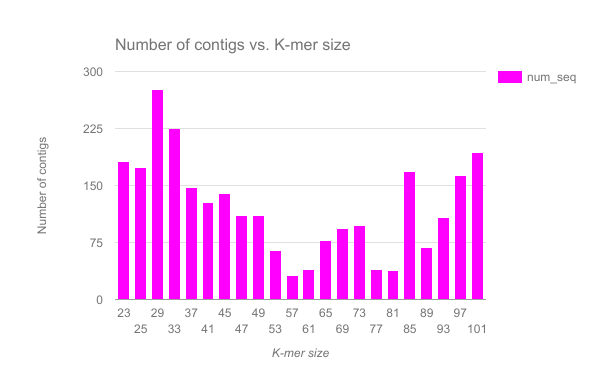
We have completed an assembly on this data set for a number of k values ranging from 29 to 101. A few of the assembly metrics appear below.

Open image in new tab

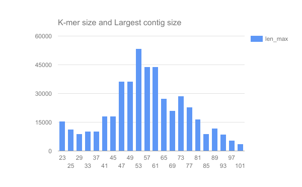Open image in new tab

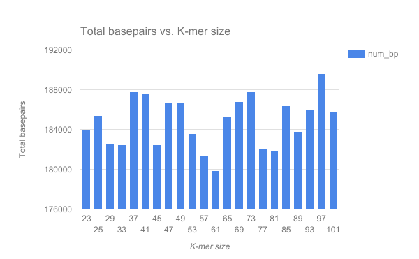Open image in new tab

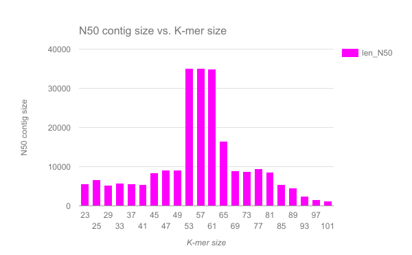Open image in new tab

Question

1. Are there any distinct features in the charts?
2. Does it look like one assembly might be better than some of the others?

The reasons for these patterns will be discussed in detail in the De Bruijn graph assembly slides and tutorial.

You've Finished the Tutorial

Please also consider filling out the Feedback Form as well!

Key points

• We assembled some Illumina fastq reads into contigs using a short read assembler called Velvet

• We showed what effect one of the key assembly parameters, the k-mer size, has on the assembly

• It looks as though there are some exploitable patterns in the metric data vs the k-mer size.

Frequently Asked Questions

Feedback

Did you use this material as an instructor? Feel free to give us feedback on how it went.
Did you use this material as a learner or student? Click the form below to leave feedback.

Citing this Tutorial

1. Simon Gladman, An Introduction to Genome Assembly (Galaxy Training Materials). https://training.galaxyproject.org/training-material/topics/assembly/tutorials/general-introduction/tutorial.html Online; accessed TODAY
2. Hiltemann, Saskia, Rasche, Helena et al., 2023 Galaxy Training: A Powerful Framework for Teaching! PLOS Computational Biology 10.1371/journal.pcbi.1010752
3. Batut et al., 2018 Community-Driven Data Analysis Training for Biology Cell Systems 10.1016/j.cels.2018.05.012

BibTeX

@misc{assembly-general-introduction,
author = "Simon Gladman",
	title = "An Introduction to Genome Assembly (Galaxy Training Materials)",
	year = "",
	month = "",
	day = "",
	url = "\url{https://training.galaxyproject.org/training-material/topics/assembly/tutorials/general-introduction/tutorial.html}",
	note = "[Online; accessed TODAY]"
}
@article{Hiltemann_2023,
	doi = {10.1371/journal.pcbi.1010752},
	url = {https://doi.org/10.1371%2Fjournal.pcbi.1010752},
	year = 2023,
	month = {jan},
	publisher = {Public Library of Science ({PLoS})},
	volume = {19},
	number = {1},
	pages = {e1010752},
	author = {Saskia Hiltemann and Helena Rasche and Simon Gladman and Hans-Rudolf Hotz and Delphine Larivi{\`{e}}re and Daniel Blankenberg and Pratik D. Jagtap and Thomas Wollmann and Anthony Bretaudeau and Nadia Gou{\'{e}} and Timothy J. Griffin and Coline Royaux and Yvan Le Bras and Subina Mehta and Anna Syme and Frederik Coppens and Bert Droesbeke and Nicola Soranzo and Wendi Bacon and Fotis Psomopoulos and Crist{\'{o}}bal Gallardo-Alba and John Davis and Melanie Christine Föll and Matthias Fahrner and Maria A. Doyle and Beatriz Serrano-Solano and Anne Claire Fouilloux and Peter van Heusden and Wolfgang Maier and Dave Clements and Florian Heyl and Björn Grüning and B{\'{e}}r{\'{e}}nice Batut and},
	editor = {Francis Ouellette},
	title = {Galaxy Training: A powerful framework for teaching!},
	journal = {PLoS Comput Biol}
}

                   

Galaxy Administrators: Install the missing tools

You can use Ephemeris's shed-tools install command to install the tools used in this tutorial.

shed-tools install [-g GALAXY] [-a API_KEY] -t <(curl https://training.galaxyproject.org/training-material/api/topics/assembly/tutorials/general-introduction/tutorial.json | jq .admin_install_yaml -r)

Alternatively you can copy and paste the following YAML

---
install_tool_dependencies: true
install_repository_dependencies: true
install_resolver_dependencies: true
tools:
- name: fastq_paired_end_interlacer
  owner: devteam
  revisions: 2ccb8dcabddc
  tool_panel_section_label: FASTA/FASTQ
  tool_shed_url: https://toolshed.g2.bx.psu.edu/
- name: fastqc
  owner: devteam
  revisions: e7b2202befea
  tool_panel_section_label: FASTA/FASTQ
  tool_shed_url: https://toolshed.g2.bx.psu.edu/
- name: fastqc
  owner: devteam
  revisions: 3d0c7bdf12f5
  tool_panel_section_label: FASTA/FASTQ
  tool_shed_url: https://toolshed.g2.bx.psu.edu/
- name: velvet
  owner: devteam
  revisions: 5da9a0e2fb2d
  tool_panel_section_label: Assembly
  tool_shed_url: https://toolshed.g2.bx.psu.edu/
- name: velvet
  owner: devteam
  revisions: 920677cd220f
  tool_panel_section_label: Assembly
  tool_shed_url: https://toolshed.g2.bx.psu.edu/
- name: velvet
  owner: devteam
  revisions: 5da9a0e2fb2d
  tool_panel_section_label: Assembly
  tool_shed_url: https://toolshed.g2.bx.psu.edu/
- name: velvet
  owner: devteam
  revisions: 920677cd220f
  tool_panel_section_label: Assembly
  tool_shed_url: https://toolshed.g2.bx.psu.edu/
- name: multiqc
  owner: iuc
  revisions: abfd8a6544d7
  tool_panel_section_label: Quality Control
  tool_shed_url: https://toolshed.g2.bx.psu.edu/
- name: multiqc
  owner: iuc
  revisions: b2f1f75d49c4
  tool_panel_section_label: Quality Control
  tool_shed_url: https://toolshed.g2.bx.psu.edu/
- name: quast
  owner: iuc
  revisions: 59db8ea8c845
  tool_panel_section_label: Assembly
  tool_shed_url: https://toolshed.g2.bx.psu.edu/
- name: quast
  owner: iuc
  revisions: 72472698a2df
  tool_panel_section_label: Assembly
  tool_shed_url: https://toolshed.g2.bx.psu.edu/

Feedback

5 stars	22
4 stars	5
3 stars	2
1 stars	2
0 stars	1

October 2024

• 4 stars: Liked: Easy to understand for non experienced

August 2024

• 4 stars: Disliked: tPlease, give more information, for exmaple to put a video or more information it was difficult to think at the end I needed to push run/play button. There is a need to indicate the files to use if there is one or multiple files.

May 2024

• 5 stars: Liked: that it explains why we are doing each step and how quality parameters should be, as well as telling you why our ensamble may be incorrect so you can correct your work Disliked: perhaps, that it could include a little bit more of theory but it was fine as it´s just a tutorial (i used this for studying really, not for practicing an assembly)

March 2024

• 5 stars: Liked: the workshop with lots of details and solution for every question Disliked: more detailed explanation about the Galaxy functions(how they work and the meaning of outputs)
• 5 stars: Liked: it is friendly, and so useful

December 2022

• 5 stars: Liked: I could follow step by step the directions Disliked: I was stacked in the velveth assembly cos I was in the wrong version of the program. Maybe is necessary to add this to the tutorial.

November 2022

• 3 stars: Liked: Everything, except the Velvet choice. Disliked: Use another software besides Velvet, since it's deprecated and it's not working.

June 2022

• 1 stars: Liked: most of the functionsare different what is given here Disliked: please insert screen shorts of the results, how the output look like

April 2022

• 5 stars: Liked: It is easy to follow up as you practice. Disliked: More examples to practice with.

March 2022

• 5 stars: Liked: Simplicity. Disliked: Considering this is an introduction to assembly, it would be helpful if the steps are complete as some steps may have been skipped. It would also be useful if pictures can be added for some steps. When ran, the results stated in this tutorial doesnt match with the output even if the instructions is strictly followed

October 2021

• 5 stars: Liked: Clarity, granularity, hands-on Disliked: Could have a similar tutorial for long read assembly (Nanopore, PB) , and I suppose 'hybrid assembly' , but this one is probably adequate for all these purposes.

February 2021

• 0 stars: Disliked: you may show the progression files in green to show us the file we have after each step i have problem with FASTQ interlacer i follow the tutorials and after this step i have two files one of them is empty and it's not working for the further stem with velveth so i'm stock at this step i don'understand why

October 2020

• 4 stars: Liked: Easy to follow Disliked: The options that appear now, are not the same that this tutorial shows.

July 2020

• 3 stars: Liked: Simple enough. Disliked: There isn't much information to give the learner the background to interpret their own data. There should be an introduction of what each of the parameters specified for the hands-on session means and why the learner should be setting them as instructed. That's the only way to know whether this tutorial is suitable for the learner's own dataset to follow.

June 2020

• 5 stars: Liked: The pace and the content covered are great!!!

April 2020

• 5 stars: Liked: the hands on exercises Disliked: There was no Icarus viewer

October 2019

• 4 stars: Liked: Step by Step instructions Disliked: Feeding in multiple samples at the same time for FastQC

June 2019

• 4 stars: Liked: the real data analysis Disliked: provide links to the tool side by side