This tutorial is not in its final state. The content may change a lot in the next months.
Because of this status, it is also not listed in the topic pages.
Single-cell RNA (scRNA) sequencing is the technological successor to classical “bulk” RNA-seq, where samples are no longer defined at the tissue level but at the individual cell level. The bulk RNA-seq methods seen in previous hands-on material would give the average expression of genes in a sample, whilst overlooking the distinct expression profiles given by the cell sub-populations due to their heterogeneity.
The rise of scRNA sequencing provides the means to explore this heterogeneity by examining samples at the individual cell level, enabling a greater understanding of the development and function of such samples, by the characteristics of their constituent cells.
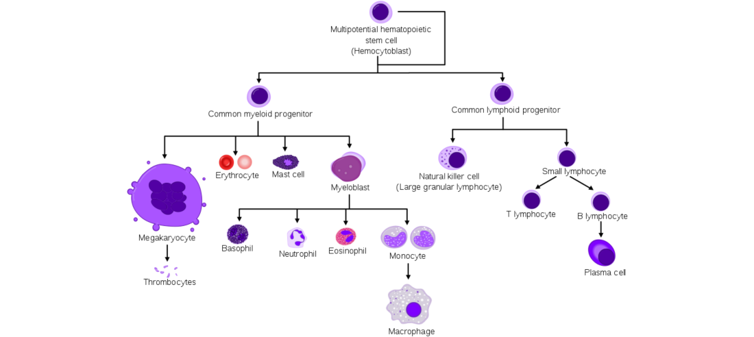
Consider the heterogeneity of cells sampled from bone marrow, where hematopoietic stem cells can give rise to many different cell types within the same tissue:
The genes expressed by these cells at different developmental time points can be subtle, but generally can be classified into discrete cell sub-populations or under statistical clustering methods such as PCA or tSNE. Cells in the same cluster exhibit similar profiles of differential expression in the same set of related genes, compared to cells in other clusters. By identifying significant genes in each cluster, cell types and cell developmental hierarchies can be inferred based on the proximity of these clusters to one another.
Other than cell development, there are many more factors that can shape the level of gene expression exhibited by a given cell. Intercellular cell-signalling can block or enhance specific transcripts, the total amount of transcripts of a cell increases with the cell-cycle, or the proximity of a cell within a tissue to nutrients or oxygen.
Most scRNA sequencing techniques use pooled-sequencing approaches to generate a higher throughput of data by performing amplification and sequencing upon multiple cells in the same “pool”. From a bioinformatics standpoint, this means that the output FASTQ data from the sequencer is batch-specific and contains all the sequences from multiple cells, where one sample of cells is equal to one batch.
In this tutorial, we will perform pre-processing upon scRNA FASTQ batch data to generate an N-by-M count matrix of N cells and M genes, with each element indicating the level of expression of that gene in a particular cell.
This count matrix is crucial for performing the downstream analysis, where differential gene analysis is performed between cells in order to cluster them into groups denoting their cell type and lineage.
The first part of this tutorial will deal with batches, and use example FASTQ data from a single batch, which we will perform barcode extraction and annotation upon. Alignment and quality control will also be performed, and we will see how to construct a rudimentary count matrix.
However, much of the essential concepts for scRNA-seq pre-processing are not explained, so it is a good idea to familiarise yourself with them in this tutorial.
The second part of this tutorial will deal with merging several output count matrices from multiple single batches generated in the first portion. Here, a set of example count matrices are merged together and quality control performed. This produces a final count matrix valid for downstream analysis.
In this tutorial we will be analysing scRNA-seq data of bone marrow cells taken from a single C57 mouse by Herman et al. (Herman et al. 2018) and producing a count matrix that we can use for later analysis.
The size of scRNA files (.fastq) are typically in the gigabyte range and are somewhat impractical for training purposes, so we will expedite the analysis by using a smaller subset of actual batch data. We will also be using Mus Musculus annotation data (.gtf) from the NCBI RefSeq track, as well as a barcodes file (.tsv).
Set the datatype of the celseq_barcodes.192.tabular to tabular
Barcode Extraction
Comment: Note
Before performing the barcode extraction process, it is recommended that you familiarise yourself with the concepts of designing cell barcodes as given by the Plates, Batches, and Barcodes, as well as the Understanding Barcodes hands-on material for an introduction into transcript barcodes.
We will be demultiplexing our FASTQ batch data by performing barcode extraction whilst also making use of the provided barcodes file to filter for specific cell barcodes.
Hands On: Barcode Extraction
UMI-tools extract ( Galaxy version 0.5.5.1) with the following parameters:
“Library type”: Paired-end Dataset Collection
param-collection“Reads in FASTQ format”: C57_P1_B1 (Our paired set)
“Barcode on both reads?”: Barcode on first read only
Verifying that the desired UMI and cell barcodes have been extracted from the sequence of the Forward reads and inserted into the header of the Reverse reads is encouraged, using the method outlined in the above hands-on material.
Question
How many reads were filtered out, and why?
The input FASTQ files contained reads from all barcodes, including those with sequencing errors, resulting in a larger pool of detected barcodes than those desired. (e.g. Cell barcode AAATTT could have single base-pair sequencing errors that could modify it into ATATTT or AAACTT, etc).
This information is included in the Log file of UMI-tools extract which contains all the parameters used to run, as well as INFO lines that indicate how many reads were read, and how many output. In this case: 134431 reads were retained (>90% of input reads).
Mapping / Alignment
FASTQ files contain sequence information that we wish to map to genes in a genome. Mapping is a relatively straightforward process, and is covered more extensively in the Sequence Analysis tutorials:
Select your genome
Select your gene annotation file
Run the alignment program
(Optional) Run MultiQC to assess the quality of the mapping
The FASTQ data was sequenced from mouse data, so to perform the alignment we will need to gather all data relevant to that genome. We will use the latest version (mm10).
The annotation GTF file must match the genome version used, since both use physical coordinates. Each GTF contains all the gene, exon, intron, and other regions of interest that we will use to annotate our reads, should our reads align to any of the regions specified in this file.
For alignment, we will use RNA-STAR for performance and splice-awareness.
Hands On: Performing the Alignment
RNA-STAR ( Galaxy version 2.7.7a) with the following parameters:
“Single-end or paired-end reads”: Single-end
param-file“RNA-Seq FASTQ/FASTA file”: Reads2 (output of UMI-tools extracttool)
“Custom or built-in reference genome”: Use a built-in index
“Reference genome with or without an annotation”: use genome reference without builtin gene-model
param-file“Gene model (gff3,gtf) file for splice junctions”: Mus_musculus.GRCm38.93.mm10.UCSC.ncbiRefSeq
MultiQC ( Galaxy version 1.9) with the following parameters:
“Results”:
“1: Results”:
“Which tool was used to generate logs?”:STAR
“STAR output”:
“1: STAR output”
“Type of STAR output?”:Log
“STAR log output” :(Select the STAR output file that ends in “log”)
Click on the galaxy-eye symbol on the MultiQC Webpage
The purpose of MultiQC is to observe how well our reads were mapped against the reference genome. Many reads are discarded due to being of too low quality, or having ambiguous sequence content that can map them to multiple locations.
Question
What percentage of our reads are uniquely mapped? How many millions of reads is this percentage?
What percentage of our reads are mapped to more than one locus?
Is our overall mapping ‘good’ ?
59.5% or ~80k reads were successfully mapped
13.6% are multiply mapped, and 3.7% were mapped to too many loci
Multiply mapped means that a read was aligned to more than one gene
Mapped to too many loci means that a read was aligned to 10 or more loci, and should be ignored.
It depends on how good the sequencing protocol is, and how many reads in total were mapped.
90% is amazing, reserved for bulk RNA-seq which typically has high coverage
70% is weak for bulk RNA-seq, but good for single-cell RNA-seq
This a small subset of a real dataset, but one would expect that 6 million mapped reads would be enough to generate a downstream analysis.
Filtering
Before continuing let us first look back on some of the previous stages:
Comment: Recap of previous stages
Barcode Extraction:
Here we used umi_tools extract on our input forward and reverse FASTQ files, and extracted the UMI and cell barcode from the forward read sequence, and placed it into the header of both forward and reverse FASTQ files. i.e. FASTQ files → Modified FASTQ files
Mapping:
We took the sequencing data from the reverse FASTQ file (with modified headers) and aligned it to the mouse genome, using annotations presented in the GTF file for that genome. i.e. Modified FASTQ file (reverse) → BAM file
Confirming Reads in the BAM file
We now have a BAM file of our aligned reads, with cell and UMI barcodes embedded in the read headers. We also have the chromosome and base-pair positions of where these reads are aligned. The can be confirmed by peeking into the BAM file:
Hands On: Confirming the Alignment Data
Click on the galaxy-eye symbol of the BAM output from STAR.
There are many header lines that begin with @ which we are not interested in.
Look at 10th read directly below the header lines:
The fields of the BAM file can be better explained at section 1.4 of the SAM specification, but we will summarise the main fields of interest here:
SRR568..._GCATTC_CTTCGT: The readname appended by _, the cell barcode, another _, and then the UMI barcode.
16: The FLAG value
Question: What does the alignment flag value of 16 tell us about this read?
We can interactively see what the different FLAG values mean by feeding values into the SAM specification to the Picard web tool
The read aligns to the reverse strand
chr13439991: The position and base-pair of alignment of the first base of the sequence.
A series of quality fields, with the main contributors being the sequence and sequence quality strings.
NH: The number of hits for this read. If it is multiply mapped, then the number of multiples will be shown (here 1, so not multiply mapped).
HI: Which number this particular read is in the series of (potentially) multi-mapped reads (here 1, not necessarily meaning the first or ‘better’).
nM: The number of base mismatches in the alignment of this read to the reference (here 1).
Filtering the BAM File
If we perform counting on the current BAM file we will be counting all reads, even the undesirable ones such as those that did not align so optimally.
The main filtering steps performed on our reads so far have been relatively silent due to the ‘default’ parameters used.
UMI-tools Extract - Filters reads for those only with matching barcodes given by our barcodes file.
RNA-STAR - As seen in the log, we lose 25% of our reads for being too short or being multiply mapped.
Another filtering measure we can apply is to keep reads that we are confident about, e.g those with a minimum number of mismatches to the reference within an acceptable range. Specifically, we want to keep all reads that align to the forward or reverse strand that also have less that 3 mismatches to the reference, and are also mapped only once to the reference.
Hands On: Task description
Filter BAM datasets on a variety of attributes ( Galaxy version 2.4.1) with the following parameters:
param-file“BAM dataset(s) to filter”: output_bam (output of RNA STARtool)
In “Condition”:
In “1: Condition”:
In “Filter”:
In “1: Filter”:
“Select BAM property to filter on”: alignmentFlag
“Filter on this alignment flag”: 0
Click on “Insert Condition”:
In “2: Condition”:
In “Filter”:
In “1: Filter”:
“Select BAM property to filter on”: alignmentFlag
“Filter on this alignment flag”: 16
Click on “Insert Condition”:
In “3: Condition”:
In “Filter”:
In “1: Filter”:
“Select BAM property to filter on”: tag
“Filter on a particular tag”: nM:<3
(Attention! please use a lowercase ‘n’ here!)
Click on “Insert Condition”:
In “4: Condition”:
In “Filter”:
In “1: Filter”:
“Select BAM property to filter on”: tag
“Filter on a particular tag”: NH:<2
“Would you like to set rules?”: Yes
“Enter rules here”: (1 | 2) & 3 & 4
Question
Why are we filtering only for alignment flags 0 and 16?
What do the tag filters nM:<3 and NH:<2 do?
What is happening at the rules stage?
Alignment flags 0 and 16 specify that we wish to only keep reads that align to the forward and reverse strands.
We are keeping reads that have a number of mismatches (nM) to the reference of less than 3, and has a number of hits (NH) across the reference of less than 2 (i.e. it is not a multiply-mapped read).
Boolean expressions are applied that state that either conditions 1 or 2 can happen, in conjunction with rules 3 and 4 happening.
Quantification
Once we have the name of the gene for a specific read, we can count how many of those reads fall into that gene and generate a count matrix.
Counting reads is performed by two commonly-used tools:
RNA-STAR
FeatureCounts
The RNA-STAR tools has the ability to count reads as it maps them. FeatureCounts performs the same task, but is capable of counting not just at the Read level, but also at the UMI level too, such that 10 duplicate reads will be counted only once.
Unfortunately, both are currently limited to counting without being able to distinguish between different cells.
If we consider the number of reads that align to GeneA, the output given by these two tools is as follows:
(reads)
RNA STAR
FeatureCounts
GeneA
12
12
But what we actually require is:
(reads)
C1
C2
GeneA
10
2
or more specifically:
(UMIs)
C1
C2
GeneA
2
1
In order to obtain this desired format, we must use UMI-tools count to perform the counting. However, this tool is dependent on FeatureCounts to annotate our reads with the one crucial piece of information that is missing from our BAM file: the name of the gene.
Comment: Verifying missing gene name
You can check this yourself by examining the galaxy-eye of the BAM file “STAR Alignment file”
Annotating Gene name with FeatureCounts
Let us annotate our BAM file with desired gene tags.
Hands On: Quantification assist via FeatureCounts
FeatureCounts ( Galaxy version 2.0.1) with the following parameters:
param-file“Alignment file”: mapped_reads (output of Filter BAMtool)
“Count multi-mapping reads/fragments”: Disabled; multi-mapping reads are excluded (default)
“Exon-exon junctions”: No (default)
“Annotates the alignment file with ‘XS:Z:’-tags to described per read or read-pair the corresponding assigned feature(s).”: Yes
Examine the output BAM file
Click on the galaxy-eye for the “Feature Counts: Alignment File”
Scroll down past the header lines
Scroll horizontally to the tags, observe the new XT tag.
The XS and XT tags in the BAM file will now form the basis for counting reads.
With all the relevant data now in our BAM file, we can actually perform the counting via UMI-tools count.
Comment: Verifying added gene name
You can once again check this yourself by examining the galaxy-eye of the BAM file “STAR Alignment file”
Counting Genes / Cell
Hands On: Final Quantification
UMI-tools count ( Galaxy version 0.5.5.1) with the following parameters:
param-file“Sorted BAM file”: out_file1 (output of FeatureCountstool)
“UMI Extract Method”: Barcodes are contained at the end of the read separated by a delimiter
“Bam is paired-end”:No
“Method to identify group of reads”:Unique
“Extra Parameters”:
“Deduplicate per gene.”:XT
“Group reads only if they have the same cell barcode.”:Yes
“Prepend a label to all column headers”:No modifications
The important parameters to take note of are those given in the Extra Parameters where we specify that each of the reads with a XT:Z tag in the BAM file will be counted on a per cell basis. Reads sharing the same UMI and cell Barcodes will be de-duplicated into a single count, reducing PCR duplicate bias from the analysis.
At this stage, we now have a tabular file containing genes/features as rows, and cell labels as headers.
Question
How many genes do we have in the matrix?
How many cells?
2,140 lines
This information can be seen in the file preview window by clicking on the name of the file (NOT the galaxy-eye symbol).
180 columns (not including the first column of gene names)
The number of columns can be seen by scrolling the file preview window completely to the right. 192 cell barcodes were given, but due to the subsetted data, only 180 were detected.
The generation of a single count matrix is now complete, with the emphasis on the word single due to the fact that we often deal in multiple batches of sequencing data.
Comment: Recap of previous stages
Barcode Extraction:
Here we used UMI_tools extract on our input forward and reverse FASTQ files, and extracted the UMI and cell barcode from the forward read sequence, and placed it into the header of both forward and reverse FASTQ files. i.e. FASTQ files → Modified FASTQ files
Mapping:
We took the sequencing data from the reverse FASTQ file (with modified headers) and aligned it to the mouse genome, using annotations presented in the GTF file for that genome. i.e. Modified FASTQ file (reverse) → BAM file
Quality Filtering:
Reads with alignment mismatches greater than 2 were discarded, and only non multi-mapped reads that mapped to the forward or reverse strand were kept
Quantification:
Gene tags were added to our alignment file, and reads were grouped according those sharing the same gene tag, with further reduction performed by collapsing all reads sharing the same cell and UMI barcode to be counted only once.
This concludes the first part of the tutorial which focused on the transformation of raw FASTQ data from a single batch into a count matrix. The second part of this tutorial guides us through the process of merging multiple processed batches from the first stage, and performing qualitative filtering.
Galaxy provides a workflow that captures the process of all the above stages for a single pair of FASTQ data:
For multiple batch processing, Galaxy can make use of Nested Workflows that in this case can take in a list of input paired FASTQ data and process them in parallel.
Handling more than one batch of sequencing data is rather trivial when we take into account our main goals and requirements:
For each batch, convert FASTQ reads from into a count matrix.
Merge all count matrices into a single count matrix
The first step merely requires us to run the same workflow on each of our batches, using the exact same inputs except for the FASTQ paired data. The second step requires a minimal level of interaction from us; namely using a merge tool and selecting our matrices.
Data upload and organisation
The count matrix we have generated in the previous section is too sparse to perform any reasonable analysis upon, and constitutes data only of a single batch. Here we will use more populated count matrices from multiple batches, under the assumption that we now know how to generate each individual one of them using the steps provided in the previous section. This data is available at Zenodo.
Once again, file naming is important, and so we will rename our matrix files appropriately to the plate and batch they are supposed to originate from.
Hands On: Data upload and organisation
Create a new history and rename it (e.g. scRNA-seq multiple-batch tutorial)
Import the eight matrices (P1_B1.tsv, P1_B2.tsv, etc.) and the barcodes file from Zenodo or from the data library (ask your instructor)
Click galaxy-uploadUpload at the top of the activity panel
Select galaxy-wf-editPaste/Fetch Data
Paste the link(s) into the text field
Press Start
Close the window
As an alternative to uploading the data from a URL or your computer, the files may also have been made available from a shared data library:
Go into Libraries (left panel)
Navigate to the correct folder as indicated by your instructor.
On most Galaxies tutorial data will be provided in a folder named GTN - Material –> Topic Name -> Tutorial Name.
Select the desired files
Click on Add to Historygalaxy-dropdown near the top and select as Datasets from the dropdown menu
In the pop-up window, choose
“Select history”: the history you want to import the data to (or create a new one)
Click on Import
Rename a matrix
Click on galaxy-pencil of the P1_B1.tsv file
Set the Name field such that it is affixed with “_P1_B1” (e.g. ‘multibatch_P1_B1’)
Click Save
Repeat for all matrices
Pay attention to the Plate number which changes after Batch 4
Merging Count Matrices
Before we begin, we must consider that our matrices are not equal – e.g. Batch1 has 3 cells that describe Genes{A,B,C,D} whereas Batch2 has 4 cells that describe Genes{C,D,E}.
We have the problem that only GeneC and GeneD appear in both batches, whilst describing 7 different cells in total.
To resolve this we can perform a “Full Table Join” where the missing data for GeneE and GeneA in Batch1 and Batch2 respectively are replaced with zeroes:
For more information on table joins, see this guide
Question
Why is it required to change the column headers in the Full matrix?
Why were the cell labels in B1 and B2 the same, if they were labelling completely different cells?
Although the cell headers in each batch matrix is the same, the cells they label are not the same and need to be relabelled in the final matrix to tell us which batch they originated from.
The reason the cell headers are the same is because the cells use the same barcodes, due to fact that the same barcodes are sometimes used across different batches.
Let us now merge our matrices from different batches. In order to ensure that our batches are merged in the order that we wish, we should first create a list of datasets so that our matrices are merged in the order given by the list.
Hands On: Table Merge
Create a Dataset List
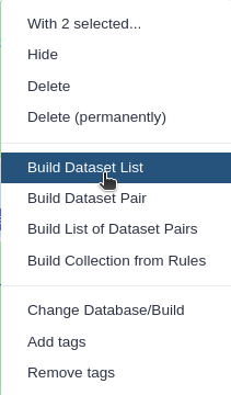
Click on galaxy-selectorSelect Items at the top of the history panel
Check all the datasets in your history you would like to include
Click n of N selected and choose Advanced Build List
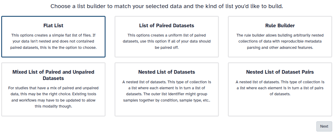
You are in collection building wizard. Choose Flat List and click ‘Next’ button at the right bottom corner.
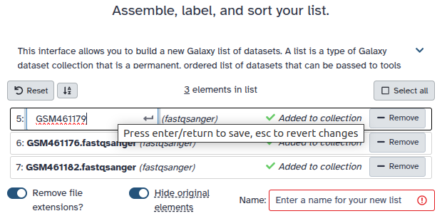
Double clcik on the file names to edit. For example, remove file extensions or common prefix/suffixes to cleanup the names.
Enter a name for your collection
Click Build to build your collection
Click on the checkmark icon at the top of your history again
Column Join on Collectionstool with the following parameters:
“Tabular Files”: (Select the Dataset Collection icon param-collection, and select the Collection from the previous step each of the matrices that you wish to join)
“Identifier column”:1
“Number of Header lines in each item”:1
“Add column name to header”:Yes
“Fill character”:0
The identifier column refers to the column where the gene names are listed. A 1:1 correspondence between matrices is checked, so that the merge does not concatenate the wrong rows between matrices. The Fill character provides a default value of 0 for cases where a Gene appears only in one of the matrices as per our example earlier.
Once the merge is complete, we can now peek at our full combined matrix by once again clicking on the file name to see a small summary.
Question
Each of these matrices/batches come from the same organism.
How much overlap in their detected genes did you expect?
How much overlap in their detected genes did you observe?
Why is this?
Given that they come from the same sample, and each matrix has ~15,000 genes, we would have expected a high overlap between matrices, yielding ~18,000 genes in the combined matrix if we assume a difference of +/- 500 genes per batch.
We observe 20,800 genes, giving less overlap between batches of the same organism than we originally thought.
The batches were sequenced at different time points along the organisms development, and therefore different genes were expressed/detected at different time points. For early development data, the overlap can be very sparse.
In the new combined matrix we see that we have 1536 cells, but this number is greatly overestimated. This is because not all batches use the same barcodes, and yet we applied the full set of 192 barcodes against our FASTQ data during the Barcode Extraction stage previously.
The reason we do this is to test for cross-contamination between batches, the details of which are better explained in the accompanying slides.
Guarding against Cross-Contamination
There are multiple possible ways to configure a plate for sequencing multiple batches. Thankfully, Galaxy provides a tool that caters for this, and checks for cross-contamination in any experimental setup. It requires only the following information:
A full list of barcodes
Which barcodes apply to which batches
Which batches apply to which plates
Since the plating protocol we are using is that designed by the Freiburg MPI Grün lab, we will follow their structure.
Barcodes:
These are each 8bp long, with an edit distance of 2, and there 192 of them.
001-006
AACACC AACCTC AACGAG AACTGG AAGCAC AAGCCA
007-012
AAGGTG AAGTGC ACAAGC ACAGAC ACAGGA ACAGTG
.
.
.
.
180-186
TTACGC TTCACC TTCCAG TTCGAC TTCTCG TTGCAC
187-192
TTGCGA TTGCTG TTGGAG TTGGCA TTGGTC TTGTGC
Plates:
Here we have 8 batches spread out over 2 plates, with alternate barcode striping.
001-096
097-192
001-096
097-192
Plate 1
B1
B2
B3
B4
Plate 2
B5
B6
B7
B8
This plating protocol can be converted into a more textual format, which allows for many variable setups (see Help section of Cross-contamination Barcode Filter tool).
“RegEx to extract Plate, Batch, and Barcodes from headers”:.*P(\\d)_B(\\d)_([ACTG]+)
“RegEx to replace Plate, Batch, and Barcodes from headers”:P\\1_B\\2_\\3
Comment: Regular Expressions
The regular expression (RegEx) used in the final steps of the above Hands-On is required in order to tell us how to capture the important information in the cell headers contained in brackets (), where \\d denotes an expected digit, and [ACTG]+ denotes 1 or more characters matching A or C or T or G.
The information captured in the brackets () can then be placed in the desired arrangement, where Place \\1 Matches \\2 Here \\3 would place the first \\d after “Place “, the second after “Matches “, and so on.
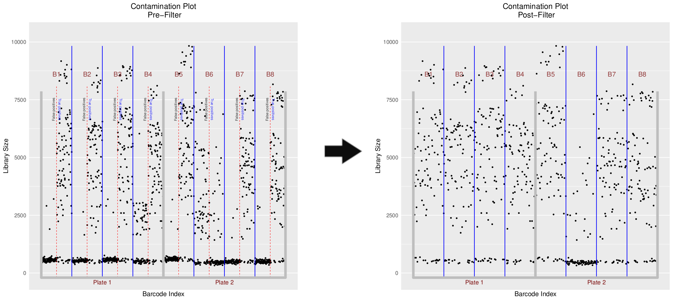
The plot that follows tells us everything we need to know about each of our batches. Each batch is essentially tested against the full set of barcodes in order to assert that only the desired or ‘Real’ barcodes have been sequenced.
In the pre-filter plot, we can see how only half of the sequences in each batch map to half the barcodes. This shows very little cross-contamination, and proves that our data is real.
The post-filter plot essentially removes the false barcodes from each batch and retains only the ‘Real’ barcodes.
Question
The count matrix that is output from this tool has only half the number of cells as the original input count matrix. Why is this?
Which batches yield worrying levels of cross-contamination?
Which batches should we remove from all further analysis?
Because only half the barcodes in each batch were real. The UMI-tools extract took the entire barcodes file to filter against each batch, and the UMI-tools count also took the entire barcodes file to count against each batch. Naturally, each batch produced 192 cells, even though 96 were real. As a result of joining each of these matrices we ended up with a count-matrix of \(8 * 192 = 1536\) cells. The cross-contamination tool removes the false barcodes (50% in each batch), resulting in \(768\) cells.
Batch 4 and Batch 6 both appear to have a significant number of mid-to-high range counts in cells under the False Positives section in these batches. This means that the cell barcodes that we should not be detecting in those batches, did in fact detect cells.
Batch 4 does still have a good number of True Positives, despite the many mid-level False Positives so we could still perhaps use the cells from that Batch. Batch 6 on the other hand appears to derive most of its counts from the False Positives, and therefore is likely not so suitable for further analysis.
All False Positives from all batches are filtered out, leaving only the True Positives (or ‘Real’ barcodes) in the remaining filtered matrix. It is up to the user to filter further based on the contamination information that they derive from this step. With this, a QC filtered count-matrix is produced that can then be used for further downstream analysis.
Conclusion
In this tutorial we have learned the importance of barcoding; namely how to define, extract, and annotate them from our reads and into the read headers, in order to preserve them during mapping. We have discovered how these barcoded reads are transformed into counts, where the cell barcode and UMI barcode are used to denote individual cells and to correct against reads that are PCR duplicates. Finally, we have learned how to combine separate batch data as well as being able to check and correct against cross-contamination.
Further information, including links to documentation and original publications, regarding the tools, analysis techniques and the interpretation of results described in this tutorial can be found here.
References
Hashimshony, T., N. Senderovich, G. Avital, A. Klochendler, Y. de Leeuw et al., 2016 CEL-Seq2: sensitive highly-multiplexed single-cell RNA-Seq. Genome Biology 17: 10.1186/s13059-016-0938-8
Herman, J. S., Sagar, and D. Grün, 2018 FateID infers cell fate bias in multipotent progenitors from single-cell RNA-seq data. Nature Methods 15: 379–386. 10.1038/nmeth.4662
Did you use this material as an instructor? Feel free to give us feedback on how it went.
Did you use this material as a learner or student? Click the form below to leave feedback.
Hiltemann, Saskia, Rasche, Helena et al., 2023 Galaxy Training: A Powerful Framework for Teaching! PLOS Computational Biology 10.1371/journal.pcbi.1010752
Batut et al., 2018 Community-Driven Data Analysis Training for Biology Cell Systems 10.1016/j.cels.2018.05.012
@misc{single-cell-scrna-preprocessing,
author = "Mehmet Tekman and Bérénice Batut and Anika Erxleben and Wolfgang Maier",
	title = "Pre-processing of Single-Cell RNA Data (Galaxy Training Materials)",
	year = "",
	month = "",
	day = "",
	url = "\url{https://training.galaxyproject.org/training-material/topics/single-cell/tutorials/scrna-preprocessing/tutorial.html}",
	note = "[Online; accessed TODAY]"
}
@article{Hiltemann_2023,
	doi = {10.1371/journal.pcbi.1010752},
	url = {https://doi.org/10.1371%2Fjournal.pcbi.1010752},
	year = 2023,
	month = {jan},
	publisher = {Public Library of Science ({PLoS})},
	volume = {19},
	number = {1},
	pages = {e1010752},
	author = {Saskia Hiltemann and Helena Rasche and Simon Gladman and Hans-Rudolf Hotz and Delphine Larivi{\`{e}}re and Daniel Blankenberg and Pratik D. Jagtap and Thomas Wollmann and Anthony Bretaudeau and Nadia Gou{\'{e}} and Timothy J. Griffin and Coline Royaux and Yvan Le Bras and Subina Mehta and Anna Syme and Frederik Coppens and Bert Droesbeke and Nicola Soranzo and Wendi Bacon and Fotis Psomopoulos and Crist{\'{o}}bal Gallardo-Alba and John Davis and Melanie Christine Föll and Matthias Fahrner and Maria A. Doyle and Beatriz Serrano-Solano and Anne Claire Fouilloux and Peter van Heusden and Wolfgang Maier and Dave Clements and Florian Heyl and Björn Grüning and B{\'{e}}r{\'{e}}nice Batut and},
	editor = {Francis Ouellette},
	title = {Galaxy Training: A powerful framework for teaching!},
	journal = {PLoS Comput Biol}
}
Funding
These individuals or organisations provided funding support for the development of this resource
3 stars:
Liked: The first section on Single Batch Processing is well-written and provides a clear explanation of the concept.
Disliked: The first section on Single Batch Processing is well-written and provides a clear explanation of the concept. However, including practical tips or guidelines for creating datasets of paired samples would be appreciated. In the second section on Multi Batch Processing, the absence of linked tools or resources is notable. As a new user, I found it challenging to locate these tools independently on the website. Providing direct links or clearer instructions for accessing the tools would significantly improve usability and accessibility for beginners.
May 2023
5 stars:
Liked: the work flow summary in a diagram format
Disliked: You could explain the steps in more detail
February 2022
5 stars:
Liked: It is very didactical
Disliked: a better explanation of cross-contamination plots
August 2021
4 stars:
Liked: The variety of tools used.
Disliked: A clearer explanation about barcodes and batches.
March 2021
0 stars:
Liked: All steps were clearly described and easily understood.
Disliked: I could not find the tool"filter bam dataset on a variety of attributes" in tool panel of Galaxy-human cell atlas , so I could not follow.
July 2019
4 stars:
Liked: Clear step-by-step instructions
Disliked: Suggestions of what to do next once the count matrix has been constructed. Can one just use standard methods such as DESeq2 for differential expression? Some examples of PCA?
Questions:
 Open image in new tab
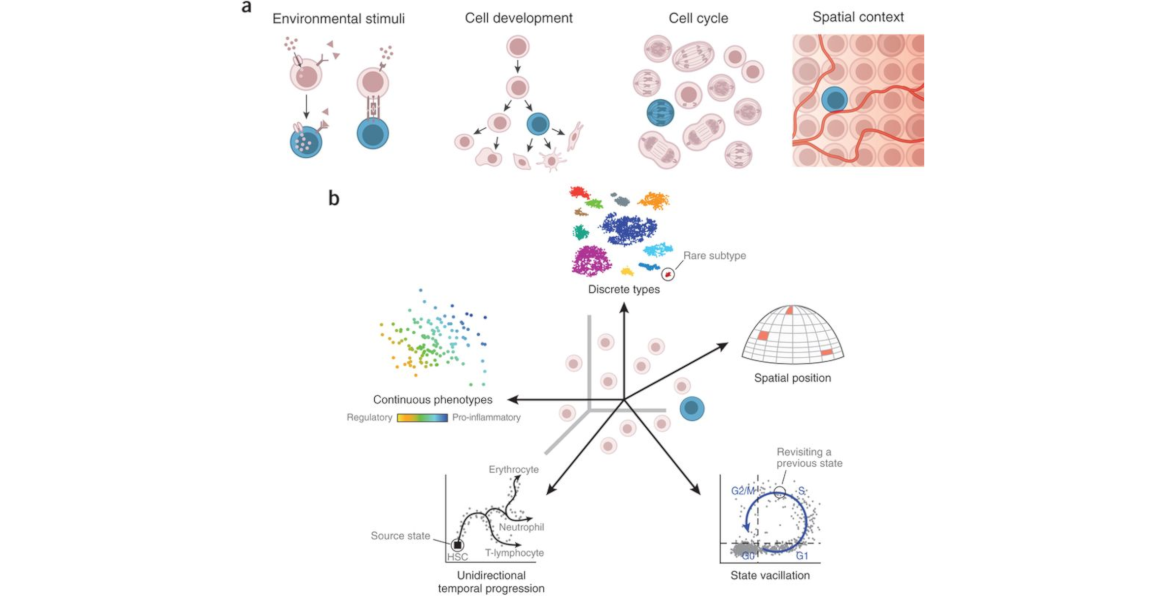 Open image in new tab
 Open image in new tab
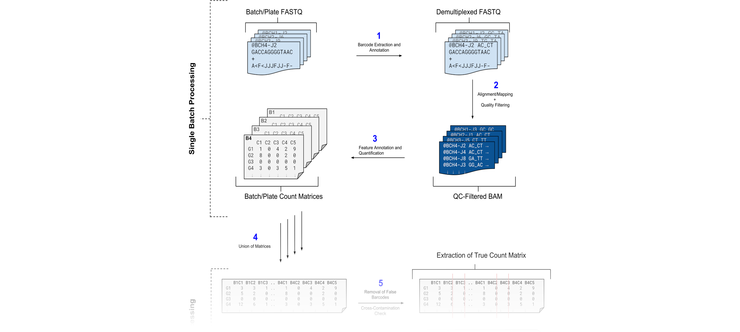 Open image in new tab

Open image in new tab
Open image in new tab
 Open image in new tab
 Open image in new tab
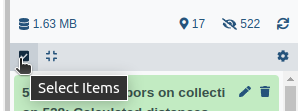
 Open image in new tab
