Where to start with bioimage analysis in Galaxy
| Author(s) |
|
| Editor(s) |
|
| Reviewers |
|
OverviewQuestions:
Objectives:
Can I process images from experimental data in Galaxy? Where do I begin?
How do I identify an image type and its metadata?
What are the basic steps of a bioimage analysis workflow?
Which workflows are best suited for my specific biological questions?
How do I choose between different segmentation strategies?
Requirements:
Classify your imaging data based on modality and dimensions (5D).
Identify the correct entry point in Galaxy (Upload vs. Bio-Formats vs. OMERO).
Apply pre-processing filters to improve data quality before analysis.
Navigate the GTN ecosystem to find specialized follow-up tutorials.
- Introduction to Galaxy Analyses
- tutorial Hands-on: FAIR Bioimage Metadata
- tutorial Hands-on: REMBI - Recommended Metadata for Biological Images – metadata guidelines for bioimaging data
Time estimation: 2 hoursLevel: Introductory IntroductorySupporting Materials:Published: Feb 17, 2026Last modification: Feb 19, 2026License: Tutorial Content is licensed under Creative Commons Attribution 4.0 International License. The GTN Framework is licensed under MITpurl PURL: https://gxy.io/GTN:T00573version Revision: 4
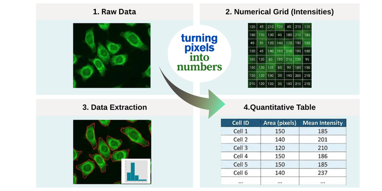
Bioimage analysis is the process of extracting meaningful information, such as quantitative data, from images in the life sciences. In this field, images are typically acquired using microscopy. Whether examining stained tissue sections in histology or tracking fluorescently labeled proteins in live cells, the fundamental goal remains consistent: turning pixels into numbers.
In Galaxy, we provide an ecosystem to make this process reproducible and scalable. We focus on making image analysis FAIR by design (Findable, Accesible, Interoperable, Reusable), ensuring that your image formats, metadata, tools, and workflows remain reusable, transparent, and traceable from the very first upload to the final figure (The Galaxy Community 2024).
This tutorial serves as your compass for navigating the Galaxy imaging landscape, specifically for bioimage data preprocessing and analysis. You will learn how image data is structured, explore the tools available in Galaxy, and discover how to kickstart your image analysis journey. By the end, you’ll understand how to transform raw, complex image data into structured tables of measurements ready for downstream statistical analysis—and know where to find the tools and resources to continue your work.
 Open image in new tab
Agenda
- 1. Know your data (the “digital anatomy” of an image)
- 2. How to get your images into Galaxy
- 3. Before you begin: diagnose your data and define your goals
- 4. The lifecycle of an analysis pipeline
- 5. Finding your workflow: modality and tools
- 6. Common pitfalls to avoid
- Conclusion
- Glossary of bioimage terms
- Next Steps: choose your tutorial
1. Know your data (the “digital anatomy” of an image)
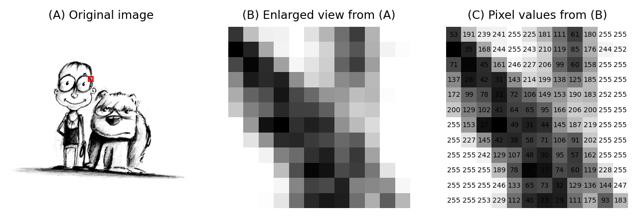
As Pete Bankhead points out in Introduction to Bioimage Analysis (Bankhead 2022), “an image is not just a picture, it is a collection of measurements.” Therefore, before starting any analysis, it is important that you understand the structure of your data.
To the human eye, an image is a visual representation of a biological sample. However, to a computer, it is a numerical array (Sedgewick and Wayne 2010). The dimensionality of this array depends on your data:
- A 2D grayscale image is a 2D array (matrix): rows × columns
- A 2D color image is a 3D array (tensor): rows × columns × channels (RGB)
- A 3D grayscale image (volume) is a 3D array: X × Y × Z
- A 3D color image (volume) is a 4D array: X × Y × Z × C
- A multi-dimensional hyperstack is a tensor: a multi-dimensional array (e.g., X × Y × Z × C × T)
Every point in that array—the pixel (2D) or voxel (3D)—is a data point representing the number of photons or the signal intensity detected at that specific coordinate. Understanding “digital anatomy” of an image means knowing exactly how those numbers were recorded, how they are organized across dimensions, how they are spaced and oriented in 3D space, and what the limitations of the employed imaging technique are (e.g., due to over/undersaturation that leads to clipped intensities).
 Open image in new tab
If you don’t understand the numbers behind the colors, you risk performing “image processing” (simply making a pretty picture) rather than “image analysis” (extracting quantitative data and meaningful insights). Let’s unpack the data behind an image step by step.
Pixels and voxels
An image is a grid of pixels (2D images) or voxels (3D images). Think of an image as a vast mosaic where every tile is a “picture element.” In 2D, these tiles are flat, but in 3D imaging, they have depth and are called voxels (“volumetric elements”, e.g., Pawley 2006). Each one is like a small bucket that has captured a specific amount of signal (usually light), which the computer records as a single number.
Image intensities represent measurements from the imaging system. To make these numbers meaningful for scientific analysis, we must define two key properties: their range (the possible values intensities can take) and their spatial extent (the physical size represented by each pixel or voxel, which determines the image resolution).
The 5 dimensions (5D)
In everyday photography, we usually deal with 2D color images. However, in the life sciences, we can capture hyperstacks: multi-dimensional data structures that represent a biological sample across space (X, Y, Z axes), spectrum (C axis), and time (T axis). Although many scientific images adopt the XYZCT (Goldberg and et al. 2005) or TCZYX axes order (e.g., (Moore and et al. 2021), making wrong assumptions about that order is a frequent source of error. It is thus important to make sure that the axes order is properly annotated in the image metadata.
- X, Y & Z (Spatial): X and Y represent the width and height of your image (the 2D plane). Z represents multiple optical sections or “slices” taken at different focal planes to reconstruct a 3D volume. In confocal or light-sheet microscopy, Z captures different depths through the sample.
- C (Channel): Different wavelengths, fluorescent probes, or staining methods corresponding to specific biological structures or molecules. In fluorescence microscopy, examples include DAPI for nuclei, GFP for proteins, and Phalloidin for actin. In histology, different channels can represent various antibody stains (immunohistochemistry) or traditional stains like hematoxylin and eosin (H&E).
- T (Time): Separate frames captured over a duration (time-lapse), allowing you to track movement, growth, or dynamic changes in cellular processes.
However, it is important to note that while we describe them in XYZCT order, different microscope vendors, tools, and file formats store them in different orders (e.g., TZCXY or XYCZT). Ensuring that the dimensional order is properly annotated within the image metadata is essential so that Galaxy (and any image analysis software in general) doesn’t accidentally interpret a Z-slice as a time-point or a channel as a Z-position (e.g., Linkert and et al. 2010).
While we often look at “merged” RGB images for presentations, you should always perform quantification on the raw, individual channels. Merging or converting to RGB often involves data compression, bit-depth reduction (typically down to 8-bit), or intensity scaling that distorts the underlying measurements and loses quantitative information (Cromey 2010). Each channel should be analyzed separately and then results can be compared or combined downstream.
Question: Identify the dimensionsIf you have a time-lapse experiment where you recorded 3 different fluorescent markers across 10 focal planes (Z-slices) every minute for an hour, how many total 2D images (planes) are in your file?
You would have: \(3 \text{ (Channels)} \times 10 \text{ (Z-slices)} \times 60 \text{ (Time points)} = 1,800 \text{ total 2D planes}\)
Each individual plane is an \(X \times Y\) image. Galaxy tools need to know the correct dimensional order (e.g.,
XYZCTvsXYCZTvsTZCXY) to ensure they correctly interpret which dimension is which—otherwise, you might accidentally measure intensity changes across Z-depth when you meant to measure changes over time!
Bit depth (the range and precision limits)
The bit depth corresponds to an upper limit of the precision when storing image intensities by determining the range of possible intensity values and the smallest distinguishable difference between them. The actual precision may also be lower and depends on many factors in your imaging system, like sensor noise, photon statistics, optical aberrations, and sample preparation quality (e.g., Pawley 2006).
When it comes to the representation of the measurements of the imaging system as the image intensities, there generally are two main types of such representation:
Integer representations
These are the natural format for raw camera data, as imaging sensors essentially count photons:
-
8-bit: 28 = 256 possible values (range: 0 to 255 for unsigned, or -128 to 127 for signed). While this looks fine to our eyes, it is often too “coarse” for thorough quantitative analysis.
-
16-bit: 216 = 65,536 possible values (range: 0 to 65,535 for unsigned, or -32,768 to 32,767 for signed). This is the scientific gold standard for image acquisition and storage, because it allows you to detect even subtle differences in image intensities that would be lost (e.g., due to rounding) when using an 8-bit representation Haase and et al. 2022.
-
32-bit: 232 = 4,294,967,296 possible values. While less common in direct acquisition, 32-bit integer formats are sometimes used in intermediate processing steps or for label images where many distinct regions need to be encoded.
Floating-point representations
After image processing operations (e.g., background subtraction, normalization, deconvolution), intensity values often become non-integer (i.e., decimal, fractional) or fall outside the original acquisition range. Floating-point formats accommodate this by representing both positive and negative values with decimal precision:
-
16-bit float (half precision): Can represent values approximately in the range of ±65,504 with limited decimal precision. This format is increasingly used in machine learning and GPU-accelerated image processing because it saves memory while providing sufficient precision for many applications.
-
32-bit float (single precision): Can represent values approximately in the range of ±1038 with about 7 significant decimal digits of precision. This is the most common format for image processing as it balances precision, range, and computational efficiency.
-
64-bit float (double precision): Can represent values approximately in the range of ±10308 with about 15-16 significant decimal digits of precision, useful for iterative algorithms or when accumulating many operations where small errors could compound.
Unlike integer representations where the precision (smallest distinguishable difference) is constant across the entire range, floating-point precision varies: it is highest near zero and decreases as values approach the limits of the representable range.
Many analysis tools automatically convert to floating-point internally to preserve accuracy during calculations.
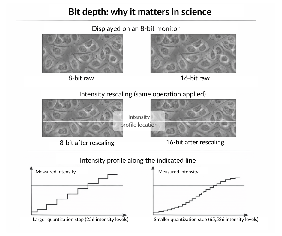
Bit depth: why it matters for science
A common misconception is that if two images look identical on a desktop monitor, they contain the same data. However, our eyes are used to computer screens that are usually limited to 8-bit, while your microscope sensor is far more sensitive.
When you perform certain pre-processing tasks, such as subtracting the image background or contrast enhancement, you are essentially stretching the histogram of the image data.
- In 8-bit, with only 256 possible values, stretching creates more pronounced “gaps” in your histogram (quantization artifacts), potentially making your data distribution appear discontinuous.
- In 16-bit integer, with 65,536 possible values, the same stretching operation creates smaller relative gaps. While quantization artifacts still occur, they are far less severe and less likely to impact downstream quantitative analysis (Cromey 2010).
The key difference is not whether artifacts appear, but their magnitude in relation to your data range. Think of it this way: spreading 256 values across a wider range creates larger “holes” between adjacent intensity levels than spreading 65,536 values across the same range.
 Open image in new tab
Always try to keep your data in 16-bit integer or floating-point formats (16-bit, 32-bit, or 64-bit float) during analysis. Converting to 8-bit too early reduces your ability to detect subtle intensity differences and makes quantization artifacts more severe during processing. This lost precision can never be recovered (Haase and et al. 2022).
Question: Why use floating-point instead of 16-bit integer?We already covered different floating-point formats in the bit depth section above. But why would we need to convert from 16-bit integer to floating-point during analysis?
16-bit integer images can only store whole numbers (0–65,535). Many image processing operations produce non-integer results that would be lost through rounding:
- Dividing pixel intensity 5 by 2 gives 2.5 (must be rounded to 2 or 3 in integer format)
- Background subtraction can produce negative values (impossible in unsigned integer format)
- Averaging two pixels with values 100 and 101 gives 100.5 (precision lost in integer)
- Normalizing intensities often produces fractional values
Floating-point still suffer from rounding but are capable to preserve these exact values with a much higher precision, reducing cumulative rounding errors across multiple processing steps. Additionally, floating-point formats can represent values in a far larger range, which is useful when processing operations produce very small or very large values (e.g., summing image intensities across multiple images; e.g., Pawley 2006). Most image analysis software automatically converts images to 32-bit float internally for this reason.
Spatial calibration (the size)
Image pixels (or voxels) have no intrinsic physical size; they are just units of storage and representation. Spatial calibration is the metadata that links these digital units to physical reality (e.g., \(1 \text{ pixel} = 0.25 \mu m\)). Without this “secret sauce,” you can count objects, but you cannot accurately measure how big they are, how fast they move, or their concentration (e.g., Linkert and et al. 2010, Haase and et al. 2022).
Metadata like the calibration information is usually stored in the image header. If you lose this metadata during a file conversion (e.g., saving as a standard .jpg), your analysis will only be able to provide quantitative results in “pixels,” which may have no biological meaning.
If you see an image intensity value of “0”, the sensor may have detected nothing, or it could represent true absence of signal—context matters. If you see the maximum value (e.g., \(255\) or \(65,535\)), your sensor was overwhelmed. These phenomena are called saturation (under- and oversaturation, respectively). Saturated pixels are often “clipped,” meaning the true biological signal was lower or higher than what the camera could record (e.g., Pawley 2006). This data is lost forever and cannot be accurately quantified.
2. How to get your images into Galaxy
Galaxy is built to handle the complexity of biological data. However, microscopy images often come in “vendor-specific” or “proprietary” formats. Your entry point into Galaxy depends on how your data was saved:
- Standard Formats (.tiff, .png): Use the standard Galaxy Upload tool.
- Open Formats: OME-TIFF, which includes standardized metadata, and OME-Zarr, a cloud-friendly image format designed to efficiently store and access very large, multi-dimensional bioimaging datasets (such as spatial transcriptomics) along with their metadata.
- Proprietary Formats (.czi, .nd2, .lif): These formats “wrap” image data and metadata together. While you can often export TIFFs from your microscope software, using the Convert image format with Bioformats ( Galaxy version 6.7.0+galaxy3) tool allows Galaxy to “unlock” and standardize the metadata hidden inside these files (Moore and et al. 2021). For more information on supported formats, see the Bio-Formats documentation.
- OMERO Integration: If your institution uses an OMERO server, you can import images directly via the Remote Files section in the upload panel. You can access OMERO using Galaxy. Additionally, you can fetch images directly using the IDR Download by IDs ( Galaxy version 0.45) tool. See Overview of the Galaxy OMERO-suite for more details.
Why use the Bio-Formats tool suite?
The Convert image format with Bio-formats ( Galaxy version 6.7.0+galaxy3) tool does more than just open a file;
Hands On: Inspecting Image Metadata
- Show image info ( Galaxy version 5.7.1+galaxy1) with the following parameters:
- param-file “Input image”:
Select your uploaded microscopy file- Review the output: Examine the resulting text file. Look for key metadata fields like “PhysicalSizeX” (pixel calibration) and “BitDepth”.
Example output:
Checking file format [Tagged Image File Format]
Initializing reader
TiffDelegateReader initializing /data/dnb10/galaxy_db/files/2/3/0/dataset_23048ef7-e850-41f4-9fc0-da24b2b4c36b.dat
Reading IFDs
Populating metadata
Checking comment style
Populating OME metadata
Initialization took 1.994s

Reading core metadata
filename = /data/dnb10/galaxy_db/files/2/3/0/dataset_23048ef7-e850-41f4-9fc0-da24b2b4c36b.dat
Series count = 1
Series #0 :
	Image count = 1
	RGB = true (3)
	Interleaved = false
	Indexed = false (false color)
	Width = 2752
	Height = 2208
	SizeZ = 1
	SizeT = 1
	SizeC = 3 (effectively 1)
	Thumbnail size = 128 x 102
	Endianness = intel (little)
	Dimension order = XYCZT (certain)
	Pixel type = uint8
	Valid bits per pixel = 8
	Metadata complete = true
	Thumbnail series = false
	-----
	Plane #0 <=> Z 0, C 0, T 0


Reading global metadata
BIG_TIFF: false
BitsPerSample: 8
Compression: LZW
DATE_TIME_DIGITIZED: 2023:07:31 16:51:32
DATE_TIME_ORIGINAL: 2023:07:31 16:51:32
ImageLength: 2208
ImageWidth: 2752
LITTLE_ENDIAN: true
MetaDataPhotometricInterpretation: RGB
MetaMorph: no
NewSubfileType: 0
NumberOfChannels: 3
PhotometricInterpretation: RGB
PlanarConfiguration: Chunky
Predictor: No prediction scheme
ResolutionUnit: Inch
SUB_SEC_TIME_DIGITIZED: 00
SUB_SEC_TIME_ORIGINAL: 00
SamplesPerPixel: 3
Software: ZEN 3.1 (blue edition)
XResolution: 300.0
YResolution: 300.0

Reading metadata
Comment: Why check this first?Before starting a long analysis, this tool helps you verify if Galaxy correctly “unlocked” the metadata inside your proprietary file. If pixel sizes are missing here, your final results will be in pixels rather than biological units like micrometers (\(\mu m\)).
For modern, large-scale, or cloud-based datasets, you can use Convert to OME-Zarr with Bio-formats ( Galaxy version 0.7.0+galaxy3). This converts a wide range of formats into OME-Zarr following the OME-NGFF specification. OME-Zarr is specifically optimized for high-performance viewing and is a staple for massive datasets like those found in spatial transcriptomics.
While there are many options, two open community-endorsed formats are increasingly dominant in bioimaging:
- OME-TIFF: Best for “classic” microscopy (2D/3D stacks) and maximum compatibility with classical software like ImageJ/Fiji or QuPath.
- OME-Zarr: A cloud-optimized format for very large, multi-dimensional bioimaging datasets (including spatial transcriptomics), enabling scalable storage and efficient data access. Moore and et al. 2021
Both are superior to proprietary formats because they make it possible to preserve your metadata attached to your pixel data throughout the entire Galaxy workflow.
Question: Metadata testingWhy we should avoid bioimages to be “Save as JPEG” from your microscope or computer?
- Data Integrity: JPEGs use “lossy” compression, which changes pixel values to save space. This approach literally modifies your scientific data.
- Metadata Retention: A standard JPEG or simple TIFF often “strips” the metadata. You would lose the information about the physical size a pixel represents, making it impossible to calculate the size of your objects later.
3. Before you begin: diagnose your data and define your goals
The first step in any analysis is to characterize the data you have. Before clicking any tools, ask yourself these four questions:
- What was the imaging modality? (Fluorescence microscopy, brightfield histology, high-content screening?)
- What is the biological subject? (Individual cells, complex tissues, or subcellular structures?)
- What is the file format? (Standard formats like .tif and .png, or proprietary vendor formats like .czi, .nd2, or .lif?)
- Where is the data stored? (A local drive, an OMERO server, a public repository, or a remote URL?)
Then, define your quantitative goals:
- What do you want to measure? (Cell count? Nuclear size? Protein intensity? Colocalization? Movement over time?)
- What level of detail do you need? (Measurements per object, summary statistics across many objects, or maps of where things are located?)
- What comparison will you make? (Differences between conditions, changes across time, or descriptive characterization?)
Depending on your answers, your starting path in Galaxy will change.
4. The lifecycle of an analysis pipeline
A typical project in Galaxy is not a single click, but a sequence of logical steps. Think of it as a factory assembly line: you start with raw materials (pixels) and move through various stations until you have a finished product (a table of measurements). Let’s examine these stages together.
Stage A: Pre-processing (cleaning)
Raw images are rarely perfect. They often contain electronic noise from the camera, uneven illumination from the microscope, or staining artifacts. Pre-processing prepares your digital image for analysis by enhancing the structures you want to identify and suppressing unwanted features like noise or artifacts (Bankhead 2022).
- Background subtraction: Removes the “haze” or background fluorescence caused by out-of-focus light. This is crucial for accurate intensity measurements later on.
- Denoising: Applies linear or non-linear filters to reduce noise while preserving meaningful structures. A Gaussian filter is a linear method that performs spatially weighted averaging using a kernel whose coefficients decrease smoothly with distance from the center, following a Gaussian (bell-shaped) distribution. It is well suited for reducing noise that approximates additive white Gaussian noise (AWGN). In contrast, a Median filter is a non-linear method that replaces each pixel value with the median of its local neighborhood. It is particularly effective for removing impulse noise such as salt-and-pepper noise and can also help mitigate impulse-like components of Poisson (shot) noise. It is also appropriate for smoothing binary or label images because it preserves original intensity values. Compared to Gaussian smoothing, median filtering better maintains sharp edges such as cell boundaries (e.g., Haase and et al. 2022).
Every filter you apply changes the pixel values. While this is necessary for segmentation, you must document these steps to ensure reproducibility. In Galaxy, this is done automatically by your history, which records every parameter used in your pre-processing steps.
In Galaxy, you can start the pre-processing stage with tools like Apply standard image filter ( Galaxy version 1.16.3+galaxy1).
Hands On: Filtering Noise
- Apply standard image filter ( Galaxy version 1.16.3+galaxy1) with the following parameters:
- param-select “Type of image data to process”:
2-D image data (or series thereof)
- param-file “Input image (2-D)”:
your_uploaded_image.tif- param-select “Filter type”:
Median
- param-text “Size”:
3Comment: Choosing the right filterTry running this tool twice: once with a Median filter (using a small Size like 3) and once with a Gaussian filter (adjusting Sigma). Zoom in on the edges of your objects. You will notice that the Median filter preserves boundaries much better, while the Gaussian filter blurs them.
Stage B: Segmentation (defining objects)
This is the most critical step. Here, you tell the computer which pixels belong to an “object” (like a nucleus) and which belong to the “background.”
- Thresholding: A “cutoff” method where pixels above (or below) a certain intensity value are classified as object. This value can be set manually or determined automatically using algorithms like Otsu or Li. The result is typically a Binary Mask.
- Inference (Deep Learning): Advanced AI models like Cellpose use pre-trained neural networks to recognize complex shapes. These methods might be superior at specific segmentation tasks such as “untangling” cells that are touching or overlapping in high-density environments (Stringer and Pachitariu 2025, Schmidt et al. 2018, Pachitariu et al. 2025).
Hands On: Creating a Segmentation Mask
- Threshold image ( Galaxy version 0.25.2+galaxy0) with the following parameters:
- param-file “Input image”:
your_filtered_image.tif- param-select “Thresholding method”:
Globally adaptive / Otsu
- param-text “Offset”:
0- param-check “Invert output labels”:
No- Review the output: You should now have a binary image where your biological objects are represented as white pixels (255) on a black background (0).
Comment: Masks vs. Label ImagesIt is important to distinguish between these two types of images in Galaxy:
- Binary Mask: This is what you created with the Threshold tool. Every pixel is either “Background” (0) or “Foreground” (255). It tells the computer where the objects are, but it doesn’t know that one cell is different from the one next to it.
- Label Image: Tools like Label objects (Connected Component Analysis) take a mask and assign a unique integer to every separate “blob.” The first cell’s pixels all become
1, the second cell2, and so on.
Stage B.1: The Region of Interest (ROI)
Once you have segmented your image, you have created Regions of Interest (ROIs). This is a central concept in bioimaging. An ROI is a spatial selection that tells the software: “Ignore the background; only calculate values for these specific coordinates.”
In Galaxy, ROIs can take three forms depending on the tool you use:
- Bounding Boxes: Simple rectangles used to crop an image or define a search area. In Galaxy, this is only possible to perform this step using interactive tools like QuPath.
- Binary Masks: A “stencil” where the ROI is white and everything else is black.
- Label Images: A “smart map” where every individual ROI has its own unique integer ID (e.g., Tosi 2021).
Comment: ROIs in interactive vs. automated toolsInteractive tools like QuPath allows users to inspect images and create ROIs either manually (e.g. drawing with the mouse) or through built-in detection algorithms that generate ROIs automatically. In automated Galaxy workflows, algorithms like Cellpose generate thousands of ROIs programmatically in a fully reproducible pipeline without user interaction (Stringer and Pachitariu 2025, Pachitariu et al. 2025).
Stage C: Post-processing (Refining)
Computers are literal; they might detect tiny specs of dust as “cells.” Post-processing is your “cleanup crew” for the mask you created in Stage B.
- Size filtering: Automatically removing any detected objects that are too small (noise) or too large (clumps of cells) to be biologically relevant.
- Morphological operations: Using operations like “Fill Holes” to fix gaps inside a detected cell or “Erode/Dilate” to slightly adjust the boundaries.
Stage D: Quantification (Extracting numbers)
Now that you have a clean mask, Galaxy “overlays” it back onto your original raw image. Since the computer knows exactly which pixels belong to which cell, it can now do the math:
- Intensity: “How much protein (fluorescence) is inside this specific mask?”
- Morphology: “How large, round, or elongated is this nucleus?”
- Spatial distribution: “How far is the nucleus from the cell membrane?”
Stage E: Validation (The sanity check)
Never trust an algorithm blindly. The final step is a visual inspection to ensure your numerical outputs represent biological reality rather than processing artifacts (Bankhead 2022).
-
Overlay outlines ( Galaxy version 3.1.9+galaxy1): This tool takes your original image and draws the boundaries of your detected objects (from your Label Image) on top of it as colored lines. It is the gold standard for visual validation, allowing you to confirm that the computer’s segmentation accurately followed the biological edges of your cells. For a detailed guide on visualizing results, see the “Visualizing Results” section in level Object Tracking using CellProfiler.
-
Overlay images ( Galaxy version 0.0.5): A versatile tool for visualizing colocalization or blending two different channels to see where biological signals overlap.
-
Render 3-D image data ( Galaxy version 0.2.0+galaxy2): For 3-D images, this tool provides similar visualization functionality, allowing you to render and inspect volumetric data.
If your segmentation (Stage B) is poor, your quantification (Stage D) will be meaningless. Always spend the most time optimizing your segmentation and validating it visually before trusting the final spreadsheet of numbers (Haase and et al. 2022).
Question: Mask vs. ImageIf you calculate the Mean Intensity of a cell, should you use the pixels from the Binary Mask or the Raw Image?
You must use the Raw Image. The mask is just a “stencil” or a map that tells the computer where to look. The actual biological information (the intensity values) is only found in the original, unprocessed image.
5. Finding your workflow: modality and tools
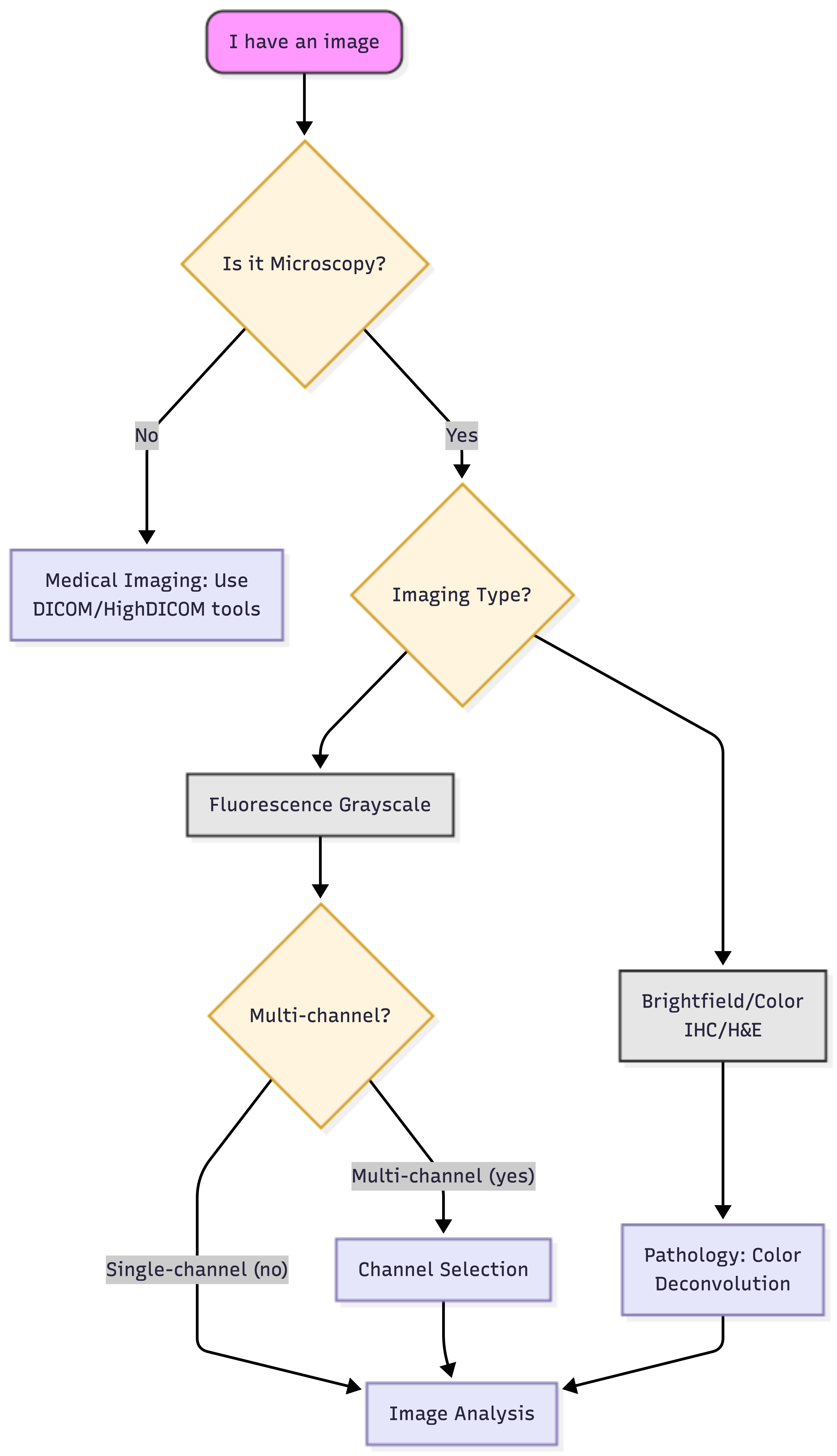
Bioimage analysis is not “one size fits all.” Galaxy provides a diverse suite of tools, from classical computer vision to state-of-the-art Deep Learning. Use the logical roadmap below to identify your specific path.
The decision tree: your logical roadmap
 Open image in new tab
The Galaxy imaging toolbox
Once you have identified your path on the tree, use this guide to find the corresponding tools in Galaxy. We categorize these into Standard Tools (for automated batch processing) and Interactive Tools (for visual exploration).
A. Standard tools (single images, high-performance & batch)
These tools are “wrapped” in Galaxy to build individual workflows and adapt your analysis to your biological question needs.
These other set of “wrapped” tools allow you to run them on hundreds of images as part of a reproducible history.
| Tool Name | Primary Application | Key Benefit |
|---|---|---|
| Cellpose | General cellular segmentation | Superior at “unsticking” crowded or overlapping cells using vector flow. |
| CellProfiler | High-content screening & automation | Allows you to build a complex multi-step “pipeline” and run it on thousands of images consistently. |
| Process image using a BioImage.IO model ( Galaxy version 2.4.1+galaxy3) | Advanced AI model inference | Gateway to the BioImage Model Zoo, run pre-trained models (like 3D U-Nets) on your data. |
Hands On: Segmentation with CellposeIn Galaxy, you can choose between the standard Cellpose model or the newer Cellpose-SAM (Segment Anything Model) version.
Option 1: Standard Cellpose
- Run generalist cell and nucleus segmentation with Cellpose 3 ( Galaxy version 3.1.0+galaxy2) with the following parameters:
- param-file “Choose the image file for segmentation”:
your_preprocessed_image.tif- param-select “Choose the pre-trained model type”:
cyto2(standard cells) ornuclei(just nuclei)- param-check “Whether to show segmentation?”:
Yes(generates a PNG preview)- In Advanced Options:
- param-text “Cell or nuclei diameter in pixels”:
Enter approximate diameter(or leave blank for automated estimation)Option 2: Cellpose-SAM (Next Gen)
- Run generalist cell and nucleus segmentation with Cellpose-SAM ( Galaxy version 4.0.8+galaxy0) with the following parameters:
- param-file “Choose the image file for segmentation”:
your_preprocessed_image.tif- param-check “Save masks as tiff?”:
Yes(Required for quantification later)- param-check “Save RGB outline images”:
Yes(Useful for Stage E: Validation)- In Advanced Options:
- param-text “Cell or nuclei diameter in pixels”:
Enter approximate diameter- param-check “Whether to use transformer backbone”:
Yes(to utilize the Cellpose3 transformer model)Comment: Multi-channel ImagesCellpose tools in Galaxy typically expect single-channel 2D images. If you have a multi-channel image, you must first use the Split image along axes tool to extract the specific channel (e.g., the DAPI channel for nuclei) that you wish to segment.
B. Interactive tools (Visual exploration)
If you prefer a “hands-on” approach to see your results in real-time before scaling up, launch an Interactive Tool (IT) directly in your browser:
- QuPath IT: The gold standard for digital pathology. Use this for large tissue sections and to access StarDist, a deep learning-based plugin for instance segmentation of star-convex shapes (e.g., nuclei), available in Galaxy through QuPath.
- Ilastik IT: Best for “training by example”—manually paint a few cells to teach the computer how to segment the rest based on texture.
- Cellpose IT: & Cellprofiler IT: Useful for building and fine-tuning your parameters visually before running a massive batch job.
Identifying your modality
To navigate the tree correctly, you must understand your image type:
-
Fluorescence: Images where pixel intensity represents the amount of light emitted. While often visualized as multi-colored immunofluorescence, the computer treats each channel as an intensity map where higher values indicate more signal.
-
Brightfield/Histology (Color): True-color images (RGB) where stains like H&E overlap. You must use Color Deconvolution to separate these into individual channels (e.g., separating Hematoxylin from DAB) before measurement. In Galaxy, you may find this tool as: Perform color deconvolution or transformation ( Galaxy version 0.9+galaxy0)
-
High-density/Tissues: For packed cells, classical thresholding fails. This is where Inference tools like Cellpose or StarDist shine, as they use pre-trained models to predict boundaries even in crowded environments. [Image comparing simple thresholding versus AI-based instance segmentation in crowded tissues]
Practice: applying the roadmap
Question: Scenario 1: The High-Volume ScreenYou have 500 images of crowded mitochondria. Which path do you choose?
You should look toward a Deep Learning approach (like Cellpose) within a CellProfiler workflow. Why?
- Crowding: Cellpose handles overlapping structures better than simple thresholding.
- Volume: With 500 images, you need the batch-processing power of CellProfiler to stay efficient.
Question: Scenario 2: The 3D VolumeYou have a single 3D Z-stack of a zebrafish embryo with one fluorescent marker. What is your path?
- Microscopy? Yes.
- Color or B&W? B&W (Single-channel fluorescence).
- Dimensionality? 3D volume. Result: You are on the Segmentation path. Use Cellpose for automated results or QuPath interactively to test different StarDist models.
6. Common pitfalls to avoid
Even with the best tools, it is easy to accidentally “break” your data before you even start measuring. In bioimage analysis, these errors are often called artifacts.
1. The “JPG” trap
Never use JPEG for science. JPEGs use “lossy” compression, meaning the computer slightly changes pixel intensities to save space. This creates “blocky” artifacts that ruin your ability to measure protein concentration or fine textures.
-
The fix: Always store quantitative microscopy data in TIFF or OME-TIFF. These formats preserve the original pixel values and metadata.
-
When is PNG OK? PNG is lossless and suitable for small 2-D single-channel or RGB images where intensities are not used for quantitative measurements. For example: 2-D label images, segmentation masks, or visualization outputs. In these cases it can reduce file size by orders of magnitude compared to TIFF. However, it should not be used for raw or measurement-grade microscopy data.
2. The “merged image” mistake
Analyzing a “Merge” (RGB) image is risky because the intensities of different channels (like DAPI and GFP) are mathematically blended into a single color value.
- The fix: Always Split Channels in Galaxy. For this purpose you may use the Split image along axes with NumPy ( Galaxy version 2.3.5+galaxy0) tool. Measure your DAPI (nuclei) and GFP (protein) separately to ensure scientific accuracy.
3. Ignoring saturation
If your image is too bright, you might hit the camera sensor’s limit (\(255\) for 8-bit or \(65,535\) for 16-bit). This is called Clipping.
- The fix: Check your histogram. If you see a giant “spike” at the very end of the graph, your data is saturated and you cannot accurately quantify the brightest parts of your sample.
Question: The artifact detectiveYou notice that in your time-lapse, the image gets slightly dimmer with every frame. Is this a biological change or an artifact?
This is likely Photobleaching, a common artifact where fluorescent molecules physically break down and lose their ability to emit light after repeated exposure to the excitation laser.
The standard approach to fix this is Bleach Correction. While a dedicated tool for this is not currently in this Galaxy workflow, you can use Perform histogram equalization ( Galaxy version 0.18.1+galaxy0) with the CLAHE algorithm as a workaround.
This does not “fix” the physical loss of signal, but it enhances the local contrast of the dim frames. This makes it possible for the segmentation tools to still detect and outline your objects in the later, darker stages of the experiment.
Conclusion
Congratulations! You have navigated the core principles of the Galaxy bioimaging landscape. By mastering these tools, you have moved beyond simply “looking” at images to performing rigorous, reproducible quantification.
In this tutorial, you have learned that:
- Images are data: Every pixel is a mathematical value. Whether you are adjusting bit depth or calibrating scales, you are ensuring that these numbers represent physical reality.
- Context matters: Using Bio-Formats and managing metadata ensures that your analysis respects the original biological dimensions, time-points, and channels.
- Segmentation is a bridge: Creating masks and label images is the critical step that allows a computer to recognize individual biological entities, such as cells or nuclei, for separate measurement.
- Validation is essential: Tools like Overlay Outlines and artifacts like Photobleaching remind us that automated analysis requires human oversight to ensure the results are biologically sound.
By building modular workflows in Galaxy, you have created a pipeline that is not only accurate but also shareable and reproducible, the gold standard of modern open science.
Further Reading
For more inspiration and a complementary perspective on designing bioimage analysis pipelines, we recommend Fazeli et al. 2025, which provides a decision tree approach to bioimage analysis that complements the workflows covered in this tutorial.
Glossary of bioimage terms
- Binary image: A black-and-white image where pixels can only have two values: 0 (Background) and 1 (Object).
- Bit depth: The number of bits used to store each pixel value, determining the range and precision of intensity values an image can represent (e.g., 8-bit = 256 values, 16-bit = 65,536 values).
- Color deconvolution: The mathematical separation of overlapping color stains (like the purple Hematoxylin and pink Eosin in H&E histology) into individual intensity channels for measurement.
- Hyperstack: A multi-dimensional image data structure that extends beyond 2D or 3D, incorporating additional dimensions such as channels (C) and time (T), typically represented as X × Y × Z × C × T.
- Label image: An image where each individual detected object is assigned a unique integer value (e.g., cell 1 = 1, cell 2 = 2), allowing the computer to distinguish and measure each object separately. Unlike a binary mask, a label image encodes object identity.
- Mask: A binary “stencil” or digital cutout that tells the computer exactly which pixels belong to an object of interest and which should be ignored.
- Metadata: Information stored alongside image data that describes how, when, and where the image was acquired (e.g., pixel size, bit depth, dimensional order, microscope settings).
- OME-TIFF: An open-source, standardized file format designed for microscopy that packages raw pixel data together with its essential metadata.
- Photobleaching: An artifact in fluorescence microscopy where fluorescent molecules permanently lose their ability to emit light after repeated exposure to the excitation laser, causing images to appear progressively dimmer over time.
- Pixel / Voxel: The smallest unit of a digital image. A pixel (2D) or voxel (3D) represents a single data point recording the signal intensity detected at a specific location in the image.
- ROI (Region of Interest): A spatial selection that defines the area of an image to be measured or analyzed, telling the software to ignore the background and focus only on specific coordinates.
- Saturation: A digital clipping artifact that occurs when light intensity exceeds the camera sensor’s maximum capacity, resulting in lost data and “flat” peaks where the brightest signals should be.
- Segmentation: The process of partitioning an image into meaningful regions by classifying pixels as belonging to either an object of interest or the background.
- Spatial calibration: Metadata that defines the physical size represented by each pixel or voxel (e.g., 1 pixel = 0.25 μm), linking digital units to real-world measurements and enabling biologically meaningful quantification.
- Thresholding: A segmentation method that classifies pixels as object or background based on whether their intensity value falls above or below a defined cutoff, producing a binary mask.
Next Steps: choose your tutorial
Now that you have your “compass,” it is time to choose a specific path. Pick the tutorial that matches your research goal:
-
The Basics: level Introduction to Image Analysis – A deeper dive into the fundamental concepts of digital images.
-
Fluorescence & Screening: level HeLa Cell Screen Analysis – Learn to process high-throughput screens using classical techniques.
-
Time-Lapse & Events: level Detection of MitoFlashes – Track transient biological events over time.
-
Classical Segmentation: level Voronoi-based Segmentation – A powerful approach for partitioning cells when they are touching but have clear centers.
-
Advanced AI: level Imaging using Bioimage Zoo Models – Use pre-trained deep learning models for complex segmentation tasks.
-
Automated Pipelines: level CellProfiler in Galaxy – Master the use of CellProfiler modules to build end-to-end automated workflows.
-
Tracking: level Object Tracking using CellProfiler – Move from static images to following individual objects through time and space.
-
Histology & Pathology: Coming Soon! A dedicated tutorial on Histology Staining and Color Deconvolution is currently in development.
You've Finished the Tutorial
Key points
Image analysis starts with understanding your metadata; pixels are just numbers with biological context.
Bioimage analysis is a multi-step pipeline, not a single tool step.
Reproducibility in Galaxy is achieved by saving every step and associated metadata in your history.
Always preserve your raw data; avoid lossy formats like JPG for analysis.
Validate your segmentation visually before trusting the numbers.
Frequently Asked Questions
Have questions about this tutorial? Have a look at the available FAQ pages and support channelsUseful literature
Further information, including links to documentation and original publications, regarding the tools, analysis techniques and the interpretation of results described in this tutorial can be found here.
References
- Goldberg, I. G., and et al., 2005 The Open Microscopy Environment (OME) Data Model and XML file: open tools for informatics and quantitative analysis in biological imaging. Genome Biology 6: R47. 10.1186/gb-2005-6-5-r47
- Pawley, J. B. (Ed.), 2006 Handbook of Biological Confocal Microscopy. Springer New York, NY. 10.1007/978-0-387-45524-2
- Cromey, D. W., 2010 Avoiding twisted pixels: ethical guidelines for the appropriate use and manipulation of scientific digital images. Science and Engineering Ethics 16: 639–667. 10.1007/s11948-010-9201-y
- Linkert, M., and et al., 2010 Metadata matters: access to image data in the real world. Journal of Cell Biology 189: 777–782. 10.1083/jcb.201004104
- Sedgewick, R., and K. Wayne, 2010 Algorithms. Addison-Wesley Professional. https://algs4.cs.princeton.edu/home/
- Schmidt, U., M. Weigert, C. Broaddus, and G. Myers, 2018 Cell Detection with Star-Convex Polygons, in Medical Image Computing and Computer Assisted Intervention – MICCAI 2018, Springer, Cham. 10.1007/978-3-030-00934-2_30
- Moore, J., and et al., 2021 OME-NGFF: a next-generation file format for expanding bioimaging data-access strategies. Nature Methods 18: 1496–1498. 10.1038/s41592-021-01326-w
- Tosi, S., 2021 Bioimage Data Analysis Workflows. Wiley-VCH. https://analyticalscience.wiley.com/do/10.1002/was.00050003/full/bioimagedataanalysis.pdf
- Bankhead, P., 2022 Introduction to Bioimage Analysis. Online. A comprehensive open-source guide to the principles of bioimage analysis.. https://bioimagebook.github.io/
- Haase, R., and et al., 2022 A Hitchhiker’s guide through the bio-image analysis software universe. FEBS Letters. 10.1002/1873-3468.14451
- The Galaxy Community, 2024 The Galaxy platform for accessible, reproducible, and collaborative data analyses: 2024 update. Nucleic Acids Research 52: W83–W94. 10.1093/nar/gkae410
- Fazeli, E., R. Haase, M. Doube, K. Miura, and D. Legland, 2025 From cells to pixels: A decision tree for designing bioimage analysis pipelines. Journal of Microscopy 300: 384–408. 10.1111/jmi.70021
- Pachitariu, M., M. Rariden, and C. Stringer, 2025 Cellpose-SAM: superhuman generalization for cellular segmentation. bioRxiv. 10.1101/2025.04.28.651001 https://www.biorxiv.org/content/early/2025/05/01/2025.04.28.651001
- Stringer, C., and M. Pachitariu, 2025 Cellpose3: one-click image restoration for improved cellular segmentation. Nature methods 22: 592–599. https://www.nature.com/articles/s41592-025-02595-5
Feedback
Did you use this material as an instructor? Feel free to give us feedback on how it went.
Did you use this material as a learner or student? Click the form below to leave feedback.

Citing this Tutorial
- Diana Chiang Jurado, Beatriz Serrano-Solano, Leonid Kostrykin, Where to start with bioimage analysis in Galaxy (Galaxy Training Materials). https://training.galaxyproject.org/training-material/topics/imaging/tutorials/where-to-start-bioimaging-galaxy/tutorial.html Online; accessed TODAY
- Hiltemann, Saskia, Rasche, Helena et al., 2023 Galaxy Training: A Powerful Framework for Teaching! PLOS Computational Biology 10.1371/journal.pcbi.1010752
- Batut et al., 2018 Community-Driven Data Analysis Training for Biology Cell Systems 10.1016/j.cels.2018.05.012
@misc{imaging-where-to-start-bioimaging-galaxy,
author = "Diana Chiang Jurado and Beatriz Serrano-Solano and Leonid Kostrykin",
	title = "Where to start with bioimage analysis in Galaxy (Galaxy Training Materials)",
	year = "",
	month = "",
	day = "",
	url = "\url{https://training.galaxyproject.org/training-material/topics/imaging/tutorials/where-to-start-bioimaging-galaxy/tutorial.html}",
	note = "[Online; accessed TODAY]"
}
@article{Hiltemann_2023,
	doi = {10.1371/journal.pcbi.1010752},
	url = {https://doi.org/10.1371%2Fjournal.pcbi.1010752},
	year = 2023,
	month = {jan},
	publisher = {Public Library of Science ({PLoS})},
	volume = {19},
	number = {1},
	pages = {e1010752},
	author = {Saskia Hiltemann and Helena Rasche and Simon Gladman and Hans-Rudolf Hotz and Delphine Larivi{\`{e}}re and Daniel Blankenberg and Pratik D. Jagtap and Thomas Wollmann and Anthony Bretaudeau and Nadia Gou{\'{e}} and Timothy J. Griffin and Coline Royaux and Yvan Le Bras and Subina Mehta and Anna Syme and Frederik Coppens and Bert Droesbeke and Nicola Soranzo and Wendi Bacon and Fotis Psomopoulos and Crist{\'{o}}bal Gallardo-Alba and John Davis and Melanie Christine Föll and Matthias Fahrner and Maria A. Doyle and Beatriz Serrano-Solano and Anne Claire Fouilloux and Peter van Heusden and Wolfgang Maier and Dave Clements and Florian Heyl and Björn Grüning and B{\'{e}}r{\'{e}}nice Batut and},
	editor = {Francis Ouellette},
	title = {Galaxy Training: A powerful framework for teaching!},
	journal = {PLoS Comput Biol}
}
Funding
These individuals or organisations provided funding support for the development of this resource

You can use Ephemeris's
shed-tools installcommand to install the tools used in this tutorial.shed-tools install [-g GALAXY] [-a API_KEY] -t <(curl https://training.galaxyproject.org/training-material/api/topics/imaging/tutorials/where-to-start-bioimaging-galaxy/tutorial.json | jq .admin_install_yaml -r)Alternatively you can copy and paste the following YAML
---
install_tool_dependencies: true
install_repository_dependencies: true
install_resolver_dependencies: true
tools:
- name: bioimage_inference
  owner: bgruening
  revisions: d5233b9d32bb
  tool_panel_section_label: Imaging
  tool_shed_url: https://toolshed.g2.bx.psu.edu/
- name: cellpose
  owner: bgruening
  revisions: 6b840482cc25
  tool_panel_section_label: Imaging
  tool_shed_url: https://toolshed.g2.bx.psu.edu/
- name: cp_overlay_outlines
  owner: bgruening
  revisions: b44b081bcf37
  tool_panel_section_label: Imaging
  tool_shed_url: https://toolshed.g2.bx.psu.edu/
- name: 2d_auto_threshold
  owner: imgteam
  revisions: 2ee04d2ebdcf
  tool_panel_section_label: Imaging
  tool_shed_url: https://toolshed.g2.bx.psu.edu/
- name: 2d_histogram_equalization
  owner: imgteam
  revisions: b1c2c210813c
  tool_panel_section_label: Imaging
  tool_shed_url: https://toolshed.g2.bx.psu.edu/
- name: 2d_simple_filter
  owner: imgteam
  revisions: 59e9798010ce
  tool_panel_section_label: Imaging
  tool_shed_url: https://toolshed.g2.bx.psu.edu/
- name: bfconvert
  owner: imgteam
  revisions: fcadded98e61
  tool_panel_section_label: Imaging
  tool_shed_url: https://toolshed.g2.bx.psu.edu/
- name: bioformats2raw
  owner: imgteam
  revisions: d7e5cf35577d
  tool_panel_section_label: Imaging
  tool_shed_url: https://toolshed.g2.bx.psu.edu/
- name: color_deconvolution
  owner: imgteam
  revisions: 0cbdf78fee14
  tool_panel_section_label: Imaging
  tool_shed_url: https://toolshed.g2.bx.psu.edu/
- name: image_info
  owner: imgteam
  revisions: f8b4eada923c
  tool_panel_section_label: Imaging
  tool_shed_url: https://toolshed.g2.bx.psu.edu/
- name: libcarna_render
  owner: imgteam
  revisions: 8fa86f0ebca2
  tool_panel_section_label: Imaging
  tool_shed_url: https://toolshed.g2.bx.psu.edu/
- name: overlay_images
  owner: imgteam
  revisions: bc4cf90cfc3b
  tool_panel_section_label: Imaging
  tool_shed_url: https://toolshed.g2.bx.psu.edu/
- name: split_image
  owner: imgteam
  revisions: 390943df8a35
  tool_panel_section_label: Imaging
  tool_shed_url: https://toolshed.g2.bx.psu.edu/
- name: idr_download_by_ids
  owner: iuc
  revisions: f92941d1a85e
  tool_panel_section_label: Imaging
  tool_shed_url: https://toolshed.g2.bx.psu.edu/