Deep learning models are increasingly used in bioimage analysis to perform processing steps such as segmentation, classification, and restoration tasks (e.g., Moen et al. 2019). The BioImage Model Zoo, (BioImage.IO)(Wei et al. 2021) is a repository that provides access to pre-trained AI models, sharing a common metadata model that allows their reuse in different tools and platforms.
Each model in BioImage.IO is tailored for a specific biological task — for example, segmenting nuclei, detecting mitochondria, or identifying neuronal structures — and trained on specific imaging modalities such as electron or fluorescence microscopy (e.g., von Chamier et al. 2021, Gómez-de-Mariscal et al. 2021).
This tutorial will guide you through the process of applying one of these BioImage.IO models to an input image using Galaxy (Batut et al. 2018). You will learn how to upload and configure the model, set the correct input parameters, and interpret the output files.
The same BioImage.IO model and the same Galaxy workflow can be applied to images from very different scientific domains. This tutorial can be followed with a bioimaging image (cell nuclei) or an Earth-observation image (lakes in a satellite scene). Only the input image changes — the model and the analysis steps are identical. Choose the path that interests you most.
Hands-on: Choose Your Own Tutorial
This is a 'Choose Your Own Tutorial' (CYOT) section (also known as 'Choose Your Own Analysis' (CYOA)), where you can select between multiple paths. Click one of the buttons below to select how you want to follow the tutorial
Pick a dataset: a fluorescence-microscopy image of cell nuclei, or a satellite image of Arctic thermokarst ponds. The model and workflow are the same for both.
Available BioImage.IO models in Galaxy
As of the version Process image using a BioImage.IO model ( Galaxy version 2.4.1+galaxy3), only the PyTorch-based BioImage.IO models listed in the table below are compatible with the Galaxy tool:
Here we illustrate the type of information that is both useful for understanding the model’s biological context and necessary for using the Galaxy tool — specifically, the input axes and input size parameters.
In both paths of this tutorial we use the same model: 🧬 NucleiSegmentationBoundaryModel
This model segments nuclei in fluorescence microscopy images. It predicts boundary maps and foreground probabilities for nucleus segmentation, primarily in images stained with DAPI. The outputs are designed to be post-processed with methods such as Multicut or Watershed to achieve instance-level segmentation (object-based segmentation).
Comment: Reusing a bioimaging model on satellite imagery
In the Earth-observation path we apply this same nucleus-segmentation model — without any retraining — to a satellite image. This is a cross-discipline experiment from the OSCARS-FIESTA project. Why does it work? Lakes and ponds strongly absorb near-infrared (NIR) light, so in an inverted NIR band they appear as bright blobs on a dark background — morphologically much like the bright nuclei the model was trained on. The model has never seen a satellite image, yet it can delineate the water bodies. Our example is a field of thermokarst ponds on the Arctic Coastal Plain of Alaska.
You can find similar details for other models directly on BioImage.IO by viewing each model’s card. Look under the “inputs” section of the RDF file to find the required axes and input size values. These parameters are essential for running the model correctly in Galaxy.
Get the data
The same BioImage.IO model is used for both paths; only the input image differs.
Hands On: Upload the model
Create a new history for this tutorial.
To create a new history simply click the new-history icon at the top of the history panel:
Import the BioImage.IO model from the Galaxy file repository:
Click on Upload Data
Go to the Choose from repository tab
Navigate to: ML models → bioimaging-models
Select nucleisegmentationboundarymodel.pt
Click Import to add it to your history
If you are importing the model from the shared data library:
As an alternative to uploading the data from a URL or your computer, the files may also have been made available from a shared data library:
Go into Libraries (left panel)
Navigate to the correct folder as indicated by your instructor.
On most Galaxies tutorial data will be provided in a folder named GTN - Material –> Topic Name -> Tutorial Name.
Select the desired files
Click on Add to Historygalaxy-dropdown near the top and select as Datasets from the dropdown menu
In the pop-up window, choose
“Select history”: the history you want to import the data to (or create a new one)
Click on Import
Rename galaxy-pencil the dataset BioImage.IO model and confirm its datatype is pt.
Click on the galaxy-pencilpencil icon for the dataset to edit its attributes
In the central panel, click galaxy-chart-select-dataDatatypes tab on the top
In the galaxy-chart-select-dataAssign Datatype, select datatypes from “New Type” dropdown
Tip: you can start typing the datatype into the field to filter the dropdown menu
Click the Save button
Now download the image for your chosen path.
Hands On: Upload the image — bioimaging
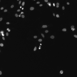
Import this fluorescence-microscopy image of cell nuclei into your history:
Click galaxy-uploadUpload at the top of the activity panel
Select galaxy-wf-editPaste/Fetch Data
Paste the link(s) into the text field
Press Start
Close the window
Rename galaxy-pencil the dataset Test image and confirm its datatype is png.
Comment: How the satellite image was prepared
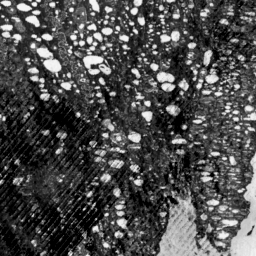
The model expects a 256×256 single-channel image. This one was built from a cloud-masked, peak-summer Landsat surface-reflectance composite of the Alaska Arctic Coastal Plain: we took the near-infrared band (in which open water is dark) and inverted it, so that water reads as bright objects on a dark background — exactly the contrast a nucleus model expects. The preprocessing notebooks, the full Galaxy run provenance, and a citable archive are in the OSCARS-FIESTA example repository.
Run the model on your image
The model run is identical for both paths.
Hands On: Run BioImage.IO model
Process image using a BioImage.IO model ( Galaxy version 2.4.1+galaxy3) with the following parameters:
param-file“BioImage.IO model”: BioImage.IO model
param-file“Input image”: Test image
param-text“Size of the input image”: 256,256,1,1
param-select“Axes of the input image”: Four axes (e.g., bcyx, byxc)
Comment: Axes and size
The param-text“Size of the input image” and the param-select“Axes of the input image” are crucial to transform the input image into the format that the BioImage.IO model requires. The correct values are provided in the RDF file that comes with the chosen model on BioImage.IO.
The model will process the input image and generate two outputs:
Two predicted images (written in one TIFF file)
A predicted tensor matrix (.npy)
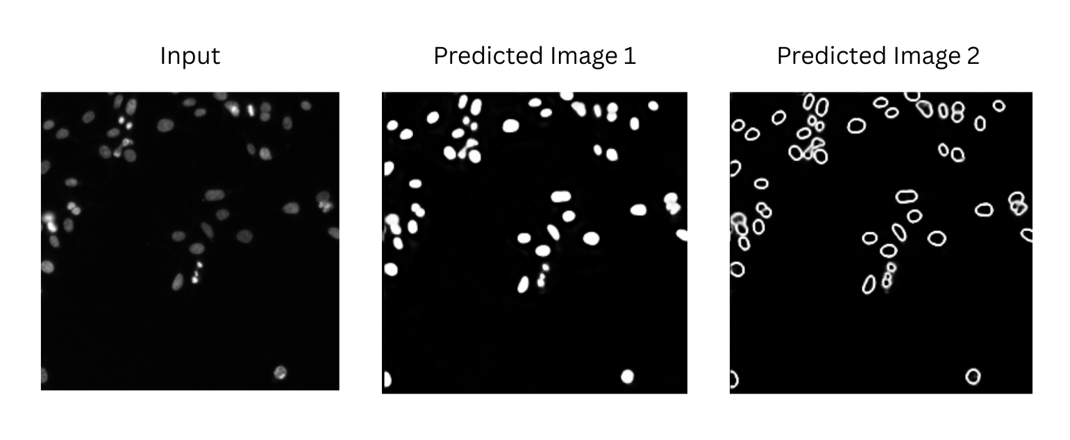
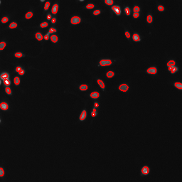
Figure 1 below is a visualization of the two predicted images generated by the 🧬 NucleiSegmentationBoundaryModel. Predicted Image 1 are the foreground probabilities and Predicted Image 2 are the boundary map.
Figure 1: The output generated by the nuclei segmentation model for the example data. The intensity values in all three images are ranging from 0 (black) to 1 (white) with gray values in between.
For the satellite image the model produces the same two channels (foreground probabilities and boundary map). After the post-processing steps below, these are combined and thresholded to delineate the water bodies — see the segmentation overlay at the end of this tutorial.
Galaxy provides a basic preview using its .tiff visualization tool. However, BioImage.IO models sometimes produce tiff files with several predicted images residing in the same tiff file.
To properly explore the results, it is recommended to click on the visualize icon in the output file, this will give you the option to display the dataset using the Avivator tool.
Figure 2: Visualize your Tiff output with Avivator in Galaxy
An alternative is to download the file and open it locally using image analysis tools such as Fiji/ImageJ, napari, or QuPath.
Question: Check your understanding
Why do the image axes matter when using a model?
What happens if the image size does not match the model input?
What are TIFF and NPY formats?
How can you interpret the output of the model, and what does it tell you about your input image?
Because deep learning models are trained on specific image shapes and dimensions; mismatches will cause errors or wrong results.
The model will fail to run or produce invalid output.
TIFF (.tiff) is a standard format for storing image data, commonly used in microscopy and bioimaging. It can be easily viewed and interpreted visually.
NPY (.npy) is a binary format used by NumPy to store arrays. In this case, it contains the raw prediction tensor produced by the model, which can be useful for further analysis or visualization with Python tools.
The model generates a predicted image that highlights or segments specific structures (e.g. nuclei, cells, mitochondria) based on what it learned during training. By comparing the output image to the input, users can see which regions were detected or classified, helping to extract biological meaning from the raw data.
Post-processing of the model output
The post-processing is the same for both paths. There are two challenges when it comes to using the model output for subsequent analysis. First, the model produces a single output file with two images (boundary maps and foreground probabilities), so for subsequent analysis we need to extract the corresponding information from that file. Second, neither of the two images produced by the model directly corresponds to segmentation results. Albeit the extracted image (Predicted Image 1) looks like a binary image with intensity 0 for the image background and intensity 1 for the image foreground, it is not. For example, there are fine contours of intensity values subtly below 1 between closely clustered cell nuclei. Thus, to obtain segmentation results, we first need to threshold the foreground probabilities (values ranging between 0 and 1) to determine the image foreground (as a binary image without any values between 0 and 1).
However, directly thresholding the foreground probabilities is going to lose information when it comes to closely clustered cell nuclei, where the crucial information is stored in the boundary map. To cope with that, we will extract both images (the foreground probabilities and the boundary map) from the output file, combine their information into a single image, and then perform thresholding.
Hands On: Extract the segmentation results from the model output
Split image along axes ( Galaxy version 2.2.3+galaxy1) with the following parameters:
param-file“Input Image”: the output from “Run BioImage.IO model”
param-select“Axis to split along”: Q-axis (other or unknown axis)
param-check“Squeeze result images”
This produces a dataset collection with two items (the two images). Next, we need to extract the first dataset (Predicted Image 1) from this collection.
Extract dataset with the following parameters:
param-file“Input List”: the output from the previous step
param-select“How should a dataset be selected”: Select by index
param-select“Element index”: 0
This will yield the file 1.tiff in your history (Predicted Image 1).
Extract dataset with the following parameters:
param-file“Input List”: the output from the previous step
param-select“How should a dataset be selected”: Select by index
param-select“Element index”: 1
This will yield the file 2.tiff in your history (Predicted Image 2).
Next, we will combine the information from the two images into a single image.
Process images using arithmetic expressions ( Galaxy version 1.26.4+galaxy2)
param-text“Expression”: foreground - boundaries
param-repeat“Input images”:
param-file“Image”: 1.tiff
param-text“Variable for representation of the image within the expression”: foreground
param-repeat“Input images”:
param-file“Image”: 2.tiff
param-text“Variable for representation of the image within the expression”: boundaries
Question
What is the motivation for combining the information from the two images with this arithmetic expression?
Each pixel of the foreground image (Predicted Image 1) corresponds to the probability of that pixel being part of a foreground object. We have also seen that the boundaries image (Predicted Image 2) uses white (intensity value 1) to encode pixels which likely correspond to boundaries of cell nuclei, and lower intensity values for others. Thus, we can interpret the boundaries image as boundary probabilities, in the sense that each pixel of that image corresponds to the probability of that pixel being part of an object boundary (i.e. the boundary of a nucleus). By considering the expression foreground - boundaries, we essentially consider the probability of each pixel being part of the image foreground, plus the probability of that point being not part of an object boundary.
Thus, in the resulting image, the intensity of each pixel pixel can be interpreted as the probability of that pixel being part of the interior of a foreground object. This better preserves information about the individual cell nuclei in the image, which is especially crucial for closely clustered cell nuclei, as opposed to considering the foregorund probabilities solely.
This interpretation also gives rise to the choice of 0.6 as the threshold value for in the next step (see below). Naturally, we would choose 0.5 to determine the image regions for which the probability is higher than 50% that the image pixels correspond to the interior of foreground objects (cell nuclei), but to improve the separation of closely clustered cell nuclei, it is a good practice to choose a threshold that is somewhat higher.
Threshold image ( Galaxy version 0.18.1+galaxy3)
param-file“Input image”: the output of the Process images using arithmetic expressions ( Galaxy version 1.26.4+galaxy2) tool
Figure 4: Overlay of the satellite image and the contours of the water bodies delineated by the BioImage.IO nucleus-segmentation model — 152 ponds detected on this scene.
On this scene the model delineates 152 distinct water bodies. In the OSCARS-FIESTA study, the segmented water area agreed with the standard remote-sensing water index (NDWI) to within about 5% on this scene, and stayed within 0.74–1.19× of NDWI across five independent scenes — a model trained only on cell nuclei, delineating lakes from space, run entirely within Galaxy.
Comment: Counting and measuring the water bodies
After thresholding, you can convert the binary image to a label map with Convert binary image to label map ( Galaxy version 0.5+galaxy0) (Connected component analysis): the number of labels is the number of water bodies, and the number of foreground pixels (times the per-pixel ground area) is the total water area.
Conclusion
In this tutorial, you learned how to run a BioImage.IO model on an image using Galaxy. By uploading a compatible model and image, setting the appropriate size and axes, and running the tool, you obtained both a predicted image and a tensor matrix representing the model output.
You also saw that the same model and the same workflow can be applied to data from a completely different discipline: a nucleus-segmentation model built for fluorescence microscopy was reused, unchanged, to delineate lakes in a satellite image. This cross-discipline reuse is exactly what FAIR, well-described workflows and models make possible — the metadata (input axes, size, modality) travels with the model, so software from one field can be picked up and run in another.
This provides a fast, reproducible way to apply deep learning models to images — within and across scientific domains — all within Galaxy.
You've Finished the Tutorial
Please also consider filling out the Feedback Form as well!
Key points
BioImage.IO models can be run in Galaxy using a dedicated tool
Input image and model need to be compatible in size and axes
Galaxy returns both the predicted image and its tensor as output
The same Galaxy workflow can be applied to images from different scientific domains — here a bioimaging model is reused unchanged on satellite imagery
Frequently Asked Questions
Have questions about this tutorial? Have a look at the available FAQ pages and support channels
Further information, including links to documentation and original publications, regarding the tools, analysis techniques and the interpretation of results described in this tutorial can be found here.
References
Batut, B., S. Hiltemann, A. Bagnacani, D. Baker, V. Bhardwaj et al., 2018 Community-Driven Data Analysis Training for Biology. Cell Systems 6: 752–758.e1. 10.1016/j.cels.2018.05.012
Moen, E., D. Bannon, T. Kudo, W. Graf, M. W. Covert et al., 2019 Deep learning for cellular image analysis. Nature Methods 16: 1233–1246. 10.1038/s41592-019-0403-1
Gómez-de-Mariscal, E., C. García-López-de-Haro, W. Ouyang, L. Donati, E. Lundberg et al., 2021 DeepImageJ: A user-friendly plugin to run deep learning models in ImageJ. Nature Methods 18: 1192–1195. 10.1038/s41592-021-01262-9
Wei, D., X. Yi, S. Fong, A. M. Walczak, H. A. Demirci et al., 2021 BioImage.IO: A community-driven framework for AI model sharing in bioimaging. Nature Methods 18: 1196–1199. 10.1038/s41592-021-01333-x
Chamier, L. von, R. F. Laine, J. Jukkala, C. Spahn, D. Krentzel et al., 2021 ZeroCostDL4Mic: An open platform to simplify access and use of deep-learning in microscopy. Nature Communications 12: 2276. 10.1038/s41467-021-22518-0
Feedback
Did you use this material as an instructor? Feel free to give us feedback on how it went.
Did you use this material as a learner or student? Click the form below to leave feedback.
Hiltemann, Saskia, Rasche, Helena et al., 2023 Galaxy Training: A Powerful Framework for Teaching! PLOS Computational Biology 10.1371/journal.pcbi.1010752
Batut et al., 2018 Community-Driven Data Analysis Training for Biology Cell Systems 10.1016/j.cels.2018.05.012
@misc{imaging-process-image-bioimageio,
author = "Diana Chiang Jurado and Leonid Kostrykin and Anne Fouilloux",
	title = "Using BioImage.IO models for image analysis in Galaxy (Galaxy Training Materials)",
	year = "",
	month = "",
	day = "",
	url = "\url{https://training.galaxyproject.org/training-material/topics/imaging/tutorials/process-image-bioimageio/tutorial.html}",
	note = "[Online; accessed TODAY]"
}
@article{Hiltemann_2023,
	doi = {10.1371/journal.pcbi.1010752},
	url = {https://doi.org/10.1371%2Fjournal.pcbi.1010752},
	year = 2023,
	month = {jan},
	publisher = {Public Library of Science ({PLoS})},
	volume = {19},
	number = {1},
	pages = {e1010752},
	author = {Saskia Hiltemann and Helena Rasche and Simon Gladman and Hans-Rudolf Hotz and Delphine Larivi{\`{e}}re and Daniel Blankenberg and Pratik D. Jagtap and Thomas Wollmann and Anthony Bretaudeau and Nadia Gou{\'{e}} and Timothy J. Griffin and Coline Royaux and Yvan Le Bras and Subina Mehta and Anna Syme and Frederik Coppens and Bert Droesbeke and Nicola Soranzo and Wendi Bacon and Fotis Psomopoulos and Crist{\'{o}}bal Gallardo-Alba and John Davis and Melanie Christine Föll and Matthias Fahrner and Maria A. Doyle and Beatriz Serrano-Solano and Anne Claire Fouilloux and Peter van Heusden and Wolfgang Maier and Dave Clements and Florian Heyl and Björn Grüning and B{\'{e}}r{\'{e}}nice Batut and},
	editor = {Francis Ouellette},
	title = {Galaxy Training: A powerful framework for teaching!},
	journal = {PLoS Comput Biol}
}
Funding
These individuals or organisations provided funding support for the development of this resource
Questions:


 Open image in new tab
Open image in new tab
 Open image in new tab
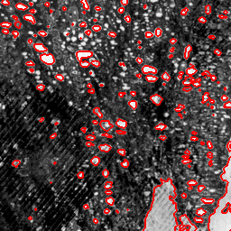 Open image in new tab