Comparative gene analysis in unannotated genomes
| Author(s) |
|
| Reviewers |
|
OverviewQuestions:
Objectives:
I have several genomes assemblies that are not annotated (or I do not trust annotations)
I am interested to compare structure of a particular gene across these genome assemblies
How do I do that?
Requirements:
Provide a quick method for identifying genes of interest in unannotated or newly assembled genomes
- Introduction to Galaxy Analyses
- tutorial Hands-on: Galaxy Basics for genomics
- tutorial Hands-on: Using dataset collections
Time estimation: 30 minutesSupporting Materials:Published: Sep 8, 2022Last modification: Jun 3, 2025License: Tutorial Content is licensed under Creative Commons Attribution 4.0 International License. The GTN Framework is licensed under MITpurl PURL: https://gxy.io/GTN:T00174rating Rating: 5.0 (0 recent ratings, 1 all time)version Revision: 10
Despite the rapidly increasing number of fully assembled genomes few genomes are well annotated. This is especially true for large eukaryotic genomes with their complex gene structure and abundance of pseudogenes. And of course do not forget about the Murthy’s law: if you are interested in a particular gene the chances are that it will not be annotated in your genome of interest. In this tutorial we will demonstrate how to compare gene structures across a set of vertebrate genomes. So …
Code In: What I have
- I know the gene’s name
- I know which species I’m interested in
- I know where to find genomes of these species
Code Out: What I want
- I work with a gene X
- I would like to compare the structure of gene X across N genomes
- Interactive graphs showing location of the gene across your species of choice. These will allow you to see the absence/presence of the genes across genomes, to detect potential duplications, predogenization events, re-arrangements etc.
- Phylogenetic trees for individual exons of the gene. The trees will give you an idea of potential unusual evolutionary dynamics for the gene.
AgendaIn this tutorial, we will deal with:
- Logic
- Example history
- Practice
- Step 1: Pick a gene and select genomes to analyze
- Step 2: Get amino acid translations for all exons of my gene of interest
- Step 3: Identify and upload genomes of interest
- Step 4: Extract amino acid sequences and genome coordinates for all ORFs
- Steps 5, 6, and 7: Finding matches and building trees
- Step 7: Looking at the trees
- Step 8: Generating and interpreting the comparative genome graph
- Interpreting the graphs
- About the gene
Logic
The analysis follow the following logic (also see the following figure):
- Pick a gene and select genomes to analyze
- Get amino acid translations for all exons of my gene of interest
- Identify genomes of interest
-
Extract amino acid sequences and genome coordinates for all possible open reading frames (ORFs) from all genomes in my set
The following steps 5, 6, and 7 are performed using a single Galaxy workflow (grey area in the following figure).
- Align - Find matches between exons of the gene of interest and ORFs
- Intersect - Compute genome coordinates of matches
-
Build phylogenetic trees for individual exons
The final step is performed using Jupyter notebook
- Create a comparative plot showing distribution of matches across genomes of interest

Example history
This example history contains results of the analysis described in this tutorial.
- Open the link to the shared history
- Click on the Import this history button on the top left
- Enter a title for the new history
- Click on Copy History
You can use this history to understand the input datasets as well as outputs of the entire analysis. The key items in the history are labelled with tags:
Code In: dataset in the example history
- EXONS - amino acid translation of exons of the gene of interest (XBP-1)
- ORF_BED - coordinates of predicted ORFs in the genomes of interest
- DiamondDB - database and amino acid translations of predicted ORFs in the genomes of interest
Code Out: in the sample history
- PlottingData - summary necessary for plotting comparative genome graphs
- Trees - phylogenetic trees for each exon
Warning: A suggestion!Importing and looking around this history is very helpful for understanding how this analysis works!
Practice
Step 1: Pick a gene and select genomes to analyze
In this example we will compare structure of X-box protein 1 gene (XBP-1) across a set of five vertebrate genomes sequenced by VGP consortium (Rhie et al. 2021).
Step 2: Get amino acid translations for all exons of my gene of interest
This step is manual and is performed outside Galaxy.
The best annotated vertebrate is … human. To obtain amino acid translation of individual exons of XBP-1 you can use UCSC Genome browser. The “UCSC annotations of RefSeq RNAs (NM_* and NR_*)” track shows two alternative transcripts produced by XBP-1 : spliced and unspliced (here ‘spliced’ and ‘unspliced’ do not refer to the “normal’ splicing process. To learn more about this fascinating gene read here).

Clicking on the names of the transcripts open a UCSC page specific to that transcript. From there you can obtain genomic sequences corresponding to all exons. You can then translate these sequences using any available online tool (e.g., NCBI ORFinder).
In this particular case we did not create translation of all exons. Instead, we created translation of exon 1 and two terminal exons. The first exon is shared between the two transcripts. It will allow us to anchor the beginning of the gene. The two terminal exons are different between the two transcripts. Because of this we create two alternative translation per exon: s-p2 and s-p12 for the spliced version and u-p1 and u-p2 for unspliced transcript. A FASTA file containing all translation is shown below:
>xbp-1u-p1
GNEVRPVAGSAESAALRLRAPLQQVQAQLSPLQNISPWILAVLTLQIQ
>xbp-1u-p2
LISCWAFWTTWTQSCSSNALPQSLPAWRSSQRSTQKDPVPYQPPFLCQWG
RHQPSWKPLMN
>xbp-1s-p12
GNEVRPVAGSAESAAGAGPVVTPPEHLPMDSGGIDSSDSE
>xbp-1s-p3
SDILLGILDNLDPVMFFKCPSPEPASLEELPEVYPEGPSSLPASLSLSVG
TSSAKLEAINELIRFDHIYTKPLVLEIPSETESQANVVVKIEEAPLSPSE
NDHPEFIVSVKEEPVEDDLVPELGISNLLSSSHCPKPSSCLLDAYSDCGY
GGSLSPFSDMSSLLGVNHSWEDTFANELFPQLISV
>xbp1_ex1
MVVVAAAPNPADGTPKVLLLSGQPASAAGAPAGQALPLMVPAQRGASPEA
ASGGLPQARKRQRLTHLSPEEKALR
Step 3: Identify and upload genomes of interest
This tutorial has been initially designed for the analysis of data produced by the Vertebrate Genome Consortium VGP. However, it is equally suitable for any genomic sequences (including prokaryotic ones).
In this section we first show how to upload sample datasets. These datasets were intentionally made small. All subsequent steps of this tutorial are performed using these sample data. We then demonstrate how to upload full size genomes from the VGP data repository called GenomeArk.
Uploading sample data
Hands On: Sample Data upload
- Create a new history for this tutorial
Import the files from Zenodo using the following URLs:
https://zenodo.org/record/7034885/files/aGasCar1.fa
https://zenodo.org/record/7034885/files/bTaeGut2.fa
https://zenodo.org/record/7034885/files/fScoJap1.fa
https://zenodo.org/record/7034885/files/mCynVol1.fa
https://zenodo.org/record/7034885/files/mHomSapT2T.fa
- Copy the link location
Click galaxy-upload Upload at the top of the activity panel
- Select galaxy-wf-edit Paste/Fetch Data
Paste the link(s) into the text field
Press Start
- Close the window

These correspond to fragments of genomes from:
aGasCar1- Gastrophryne carolinensis (Eastern narrow-mouth toad)bTaeGut- Taeniopygia guttata (Zebra finch)fScoJap- Scomber japonicus (Chub mackerel)mCynVol- Cynocephalus volans (Philippine flying lemur)mHomSap- Homo sapiens (Human)
Uploading VGP data from GenomeArk
Galaxy provides a direct connection to GenomeArk from its “Upload Data” tool. To access GenomeArk data you need to:
Hands On: Upload VGP data from GenomeArk
- Create a new history for this tutorial
Import genome assembly FASTA files from GenomeArk:
- Open the file galaxy-upload Upload Data menu
- Click on Choose remote files button at the bottom of the Upload interface
- Choose Genome Ark
- Pick assembles you would like to include in your analysis (use Search box on top)
Generally for a given species you want the assembly with the highest version number. For example, Human (Homo sapiens) had three assemblies at the time of writing:
mHomSap1,mHomSap2, andmHomSap3. PickmHomSap3in this situation.Inside each assembly folder you will see typically see different sub-folders. The one you should generally be interested in will be called
assembly_curated. Inside that folder you will typically see separate assemblies for maternal (indicated withmat) and paternal (indicated withpat) haplotypes. In the analyses here we are choosing as assembly representing heterogametic haplotype (patin the case of Human).
- Repeat this process for all assemblies you are interested in.
Combine uploaded sequences into a dataset collection
After uploading data from GenomeArk you will end up with a number of FASTA datasets in your history. To proceed with the analysis you will need to combine these into a single dataset collection:
Hands On: Combine genome assemblies into a dataset collectionTo create a collection from genome assemblies you just uploaded into GenomeArk follow the steps in the video below. Obviously, you only want to click check-boxes next to FASTA files (assemblies) you want to include and leave everything else out.
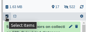
- Click on galaxy-selector Select Items at the top of the history panel
- Check all the datasets in your history you would like to include
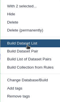
Click n of N selected and choose Advanced Build List
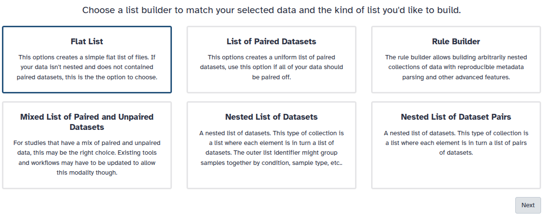
You are in collection building wizard. Choose Flat List and click ‘Next’ button at the right bottom corner.
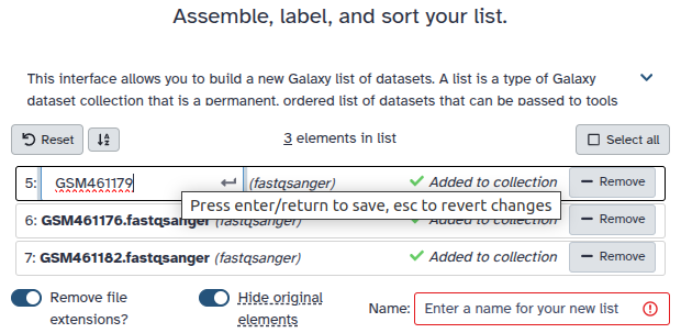
Double clcik on the file names to edit. For example, remove file extensions or common prefix/suffixes to cleanup the names.
- Enter a name for your collection
- Click Build to build your collection
- Click on the checkmark icon at the top of your history again
Step 4: Extract amino acid sequences and genome coordinates for all ORFs
Extract ORFs from genomic sequences
Now we can go ahead and find all ORFs in all genome assemblies we have bundled into a collection. For this we will use tool called ORFiPy:
Hands On: Find ORFs witrh ORFiPyRun ORFiPy ( Galaxy version 0.0.4+galaxy0) with the following parameters:
- param-collection “Find ORFs in”: The collection containing genome assemblies we just created (click “Dataset collection” param-collection button on left-side of this input field)
- “Select options”: check the box next to
BEDandPeptides- “Minimum length of ORFs”: type the number
99. We do not want ORFs to be too short as their number will be too high- “Output ORFs bound by Stop codons?”: set this option to
Yes.
Because this operation is performed on a dataset collection. it will produce a dataset collection as an output. Actually, it will produce two because we selected BED and Peptides options. One collection will contain amino acid sequences for all ORFs (it will typically be called ORFs on collection ... (FASTA format)) and another their coordinates (called ORFs on collection ... (BED format))
)
This will produce two new dataset collections in your history: one containing coordinates of ORFs and the other containing their amino acid translations. Because genomes are large these will likely be tens of millions of ORFs identified this way.
Creating Diamond database
Because we will be using the Diamond tool to find matches between our gene of interest and ORF translations we need to convert FASTA files into Diamond database using Diamond makedb tool:
Hands On: Create Diamond databaseRun Diamond makedb ( Galaxy version 2.0.15+galaxy0) on the collection containing amino acid translations of ORFs generated using ORFiPy:
- param-collection “Input reference file in FASTA format”*: Select collections containing amino acid (FASTA Protein) output of ORFiPy
At this point we have three input datasets that would allow us to find and visualize matches between the gene of interest and genome asseblies:
- Diamond database of ORF translations from genome assemblies
- Coordinates and frame information about ORFs in BED format
- Amino acid translation of exons from the gene of interest
Steps 5, 6, and 7: Finding matches and building trees
To find location of genes, we will use the following workflow that is available as a part of this tutorial. To use this workflow you need to import it into your Galaxy instance.
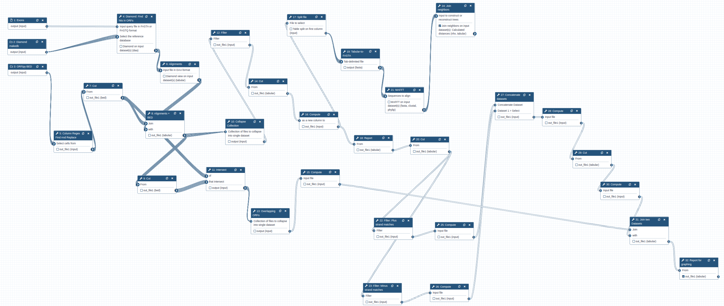
The workflow takes three inputs:
Code In: Workflow inputs
It produces two primary outputs:
Code Out: Results
- Trees - Phylogenetic trees for each input exon as Newick file
- PlottingData - A summary table of exon matches for each genome
The overall logic of the workflow is as follows:
- Perform Diamond search to identify matches between the gene of interest (EXONS) and ORF sets from each genomes (DiamondDB).
- Intersect information about the matches with BED file containing ORF coordinates (ORF BED). This allows us to know genomic position of the ORFs and their frames (1, 2, 3 or -1, -2, -3).
- Extract matching parts of the sequences and generated multiple alignments using MAFFT. This is done for each amino acid sequence in EXONS. Thus in the case of XBP-1 there will be five sets of alignments.
- Build phylogenetic tree for each alignment produced in the previous step using the Neighbor Joining method - a simple and quick way to obtain a rough phylogeny.
- Use information from step 1 to compute genome coordinates of matches. This is done by combining the information about genomic positions of ORFs from the ORF BED file and local alignment information generated during step 1.
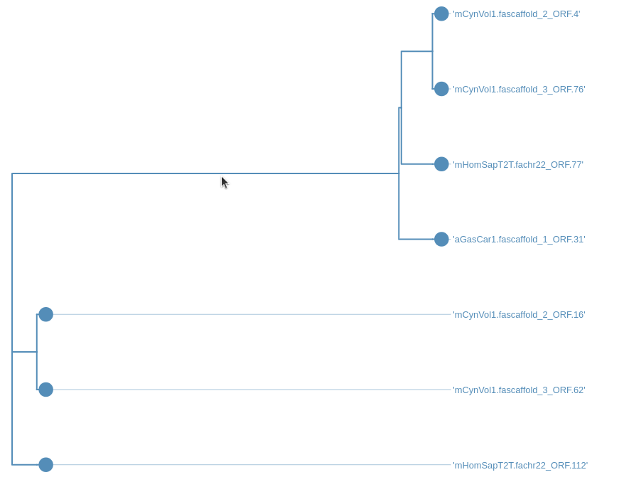
Step 7: Looking at the trees
After running the workflow phylogenetic trees will be saved into a collection named Join neighbors on .... This collection will also be labelled with tag Trees. To visualize the trees:
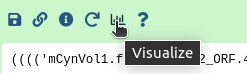
Hands On: Visualize the trees
- Expand the collection by clicking on it
- Click on any dataset
- Click the galaxy-barchart icon:
- A selection of tree visualization tools will appear in the center pane of the interface
- Select
Phylogenetic Tre Visualizationand play with it:
Step 8: Generating and interpreting the comparative genome graph
Another workflow output will represent a single file summarizing genomic location of matches between each of the genomes in our dataset and amino acid translation of exons from the gene of interest. It will be called Mapping report and will have tag PlottingData associated with it. To plot the data contained in this file we will use external Jupyter notebook (note that Jupyter can be run directly from Galaxy, but to make this tutorial runnable on any Galaxy instance we will use an internal notebook server).
Starting notebook
Hands-on: Choose Your Own TutorialThis is a 'Choose Your Own Tutorial' (CYOT) section (also known as 'Choose Your Own Analysis' (CYOA)), where you can select between multiple paths. Click one of the buttons below to select how you want to follow the tutorial
If you are on a server with Interactive Tool support (e.g. Galaxy Europe, Australia, and many others), you can choose that option for a more integrated Jupyter Notebook experience.
The notebook can be accessed from here. You do need to have a Google Account to be able to use the notebook.
Hands On: Launch JupyterLabCurrently JupyterLab in Galaxy is available on Live.useGalaxy.eu, usegalaxy.org and usegalaxy.eu.
Hands On: Run JupyterLab
- Interactive Jupyter Notebook. Note that on some Galaxies this is called Interactive JupyTool and notebook:
- Click Run Tool
The tool will start running and will stay running permanently
This may take a moment, but once the
Executed notebookin your history is orange, you are up and running!- On the left menu bar you should see the Interactive Tools Icon now. Click on it to open the Active Interactive Tools and locate the JupyterLab instance you started.
- Click on your JupyterLab instance (JupyTool interactive tool)
If JupyterLab is not available on the Galaxy instance:
- Start Try JupyterLab
-
Once the notebook has started, open a Terminal in Jupyter File → New → Terminal
-
Run the following command:
wget https://training.galaxyproject.org/training-material/topics/genome-annotation/tutorials/gene-centric/gene_image.ipynb -
Switch to the Notebook that appears in the list of files on the left
Proving data
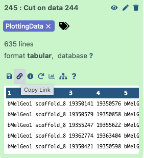
The data is provided to the notebook by setting the dataset_url parameter in this cell:
# Paste link to the dataset here
dataset_url = 'https://usegalaxy.org/api/datasets/f9cad7b01a472135a8abd43f91f8d3cf/display?to_ext=tabular'
This is a URL pointing to one of the workflow outputs: Mapping report with the PlottingData tag. To copy the URL click on the galaxy-link icon adjacent to the dataset:
Running the notebook will generate two graphs explained in the next section.
Interpreting the graphs
Analysis of sample data associated with this tutorial will produce the genome graph shown below. In this graph the Y-axis represents ORFs on positive (1, 2, 3 in red color) and negative (-1, -2, -3 in blue color) strands. The X-axis is genomic coordinates. Boxes represent matches between amino acid sequences of exons and ORFs they are superimposed to. The color of boxes reflect the extent of amino acid identity. The color key is shown in the left upper corner of the plot. The image is interactive so you can zoom in and out.
One of the interesting things you can immediate see in this graph is that the Philippine flying lemur (mCynVol) contains two copies of XBP-1 located on scaffold_2 and scaffold_3. Furthermore, the copy located on scaffold_2 looks like a retransposed duplicate of the gene because it is shorter and likely missing some of the introns – a hallmark of retrotransposition.
Another plot currently produced by the notebook is a summary plot showing the distribution of matches across species and their amino acid identity:

About the gene
XBP-1 is one of a few vertebrate gene containing overlapping reading frames encoding different proteins within a single gene (Chung et al. 2007). In this case the switch between two reading frames occurs when a highly specialized RNA endonuclease, IRE1, excises a 26 nucleotide spacer from XBP-1 mRNA (Nekrutenko and He 2006). This converts the so-called “unspliced” form of the transcript (XBP-1U) to the “spliced” form XBP-1S (Note that the term “spliced” is misleading here. The XBP-1U is already processed by splicing machinery and contains no canonical introns. The “spliced” is simply used to indicate the removal of the 26 nucleotide spacer). Because the 26 is not divisible by three, the XBP-1S transcript is translated in a different frame from the point of cleavage. The activation of IRE1 and resulting removal of the spacer is triggered by presence of unfolded proteins in the endoplasmic reticulum and the IRE1-XBP1 pathway is one of the three major unfolded protein response systems in higher eukaryotes (Chen and Cubillos-Ruiz 2021) that is conserved all the way to yeast (with XBP-1’s homologue HAC-1; Calfon et al. 2002 ) .
For questions about using Galaxy, you can ask in the Galaxy help forum.
You've Finished the Tutorial
Key points
You can locate gene of interest in unannotated genomes and compare its structure across multiple species
Frequently Asked Questions
Have questions about this tutorial? Have a look at the available FAQ pages and support channelsReferences
- Calfon, M., H. Zeng, F. Urano, and J. H. Till, 2002 IRE1 couples endoplasmic reticulum load to secretory capacity by processing the XBP-1 mRNA. ….
- Nekrutenko, A., and J. He, 2006 Functionality of unspliced XBP1 is required to explain evolution of overlapping reading frames. Trends in Genetics 22: 645–648.
- Chung, W.-Y., S. Wadhawan, R. Szklarczyk, S. K. Pond, and A. Nekrutenko, 2007 A first look at ARFome: dual-coding genes in mammalian genomes. PLoS Comput. Biol. 3: e91.
- Chen, X., and J. R. Cubillos-Ruiz, 2021 Endoplasmic reticulum stress signals in the tumour and its microenvironment. Nat. Rev. Cancer 21: 71–88.
- Rhie, A., S. A. McCarthy, O. Fedrigo, J. Damas, G. Formenti et al., 2021 Towards complete and error-free genome assemblies of all vertebrate species. Nature 592: 737–746.
Glossary
- ORF
- Open Reading Frame
Feedback
Did you use this material as an instructor? Feel free to give us feedback on how it went.
Did you use this material as a learner or student? Click the form below to leave feedback.

Citing this Tutorial
- Anton Nekrutenko, Comparative gene analysis in unannotated genomes (Galaxy Training Materials). https://training.galaxyproject.org/training-material/topics/genome-annotation/tutorials/gene-centric/tutorial.html Online; accessed TODAY
- Hiltemann, Saskia, Rasche, Helena et al., 2023 Galaxy Training: A Powerful Framework for Teaching! PLOS Computational Biology 10.1371/journal.pcbi.1010752
- Batut et al., 2018 Community-Driven Data Analysis Training for Biology Cell Systems 10.1016/j.cels.2018.05.012
Congratulations on successfully completing this tutorial!@misc{genome-annotation-gene-centric, author = "Anton Nekrutenko", title = "Comparative gene analysis in unannotated genomes (Galaxy Training Materials)", year = "", month = "", day = "", url = "\url{https://training.galaxyproject.org/training-material/topics/genome-annotation/tutorials/gene-centric/tutorial.html}", note = "[Online; accessed TODAY]" } @article{Hiltemann_2023, doi = {10.1371/journal.pcbi.1010752}, url = {https://doi.org/10.1371%2Fjournal.pcbi.1010752}, year = 2023, month = {jan}, publisher = {Public Library of Science ({PLoS})}, volume = {19}, number = {1}, pages = {e1010752}, author = {Saskia Hiltemann and Helena Rasche and Simon Gladman and Hans-Rudolf Hotz and Delphine Larivi{\`{e}}re and Daniel Blankenberg and Pratik D. Jagtap and Thomas Wollmann and Anthony Bretaudeau and Nadia Gou{\'{e}} and Timothy J. Griffin and Coline Royaux and Yvan Le Bras and Subina Mehta and Anna Syme and Frederik Coppens and Bert Droesbeke and Nicola Soranzo and Wendi Bacon and Fotis Psomopoulos and Crist{\'{o}}bal Gallardo-Alba and John Davis and Melanie Christine Föll and Matthias Fahrner and Maria A. Doyle and Beatriz Serrano-Solano and Anne Claire Fouilloux and Peter van Heusden and Wolfgang Maier and Dave Clements and Florian Heyl and Björn Grüning and B{\'{e}}r{\'{e}}nice Batut and}, editor = {Francis Ouellette}, title = {Galaxy Training: A powerful framework for teaching!}, journal = {PLoS Comput Biol} }
You can use Ephemeris's
shed-tools installcommand to install the tools used in this tutorial.shed-tools install [-g GALAXY] [-a API_KEY] -t <(curl https://training.galaxyproject.org/training-material/api/topics/genome-annotation/tutorials/gene-centric/tutorial.json | jq .admin_install_yaml -r)Alternatively you can copy and paste the following YAML
---
install_tool_dependencies: true
install_repository_dependencies: true
install_resolver_dependencies: true
tools:
- name: diamond
  owner: bgruening
  revisions: e8ac2b53f262
  tool_panel_section_label: NCBI Blast
  tool_shed_url: https://toolshed.g2.bx.psu.edu/
- name: diamond
  owner: bgruening
  revisions: e8ac2b53f262
  tool_panel_section_label: NCBI Blast
  tool_shed_url: https://toolshed.g2.bx.psu.edu/
- name: diamond
  owner: bgruening
  revisions: e8ac2b53f262
  tool_panel_section_label: NCBI Blast
  tool_shed_url: https://toolshed.g2.bx.psu.edu/
- name: split_file_on_column
  owner: bgruening
  revisions: 37a53100b67e
  tool_panel_section_label: Text Manipulation
  tool_shed_url: https://toolshed.g2.bx.psu.edu/
- name: column_maker
  owner: devteam
  revisions: 02026300aa45
  tool_panel_section_label: Text Manipulation
  tool_shed_url: https://toolshed.g2.bx.psu.edu/
- name: column_maker
  owner: devteam
  revisions: 6595517c2dd8
  tool_panel_section_label: Text Manipulation
  tool_shed_url: https://toolshed.g2.bx.psu.edu/
- name: intersect
  owner: devteam
  revisions: 69c10b56f46d
  tool_panel_section_label: Text Manipulation
  tool_shed_url: https://toolshed.g2.bx.psu.edu/
- name: tabular_to_fasta
  owner: devteam
  revisions: 0a7799698fe5
  tool_panel_section_label: FASTA/FASTQ
  tool_shed_url: https://toolshed.g2.bx.psu.edu/
- name: regex_find_replace
  owner: galaxyp
  revisions: ae8c4b2488e7
  tool_panel_section_label: Text Manipulation
  tool_shed_url: https://toolshed.g2.bx.psu.edu/
- name: orfipy
  owner: iuc
  revisions: c147914c9f02
  tool_panel_section_label: Extract Features
  tool_shed_url: https://toolshed.g2.bx.psu.edu/
- name: rapidnj
  owner: iuc
  revisions: 9f4a66e22580
  tool_panel_section_label: Evolution
  tool_shed_url: https://toolshed.g2.bx.psu.edu/
- name: collapse_collections
  owner: nml
  revisions: 90981f86000f
  tool_panel_section_label: Collection Operations
  tool_shed_url: https://toolshed.g2.bx.psu.edu/
- name: mafft
  owner: rnateam
  revisions: f1a5908ea2cb
  tool_panel_section_label: Multiple Alignments
  tool_shed_url: https://toolshed.g2.bx.psu.edu/