What are the preprocessing steps to prepare ONT sequencing data for further analysis?
How to identify pathogens using sequencing data?
How to track the found pathogens through all your samples datasets?
Objectives:
Check quality reports generated by FastQC and NanoPlot for metagenomics Nanopore data
Preprocess the sequencing data to remove adapters, poor quality base content and host/contaminating reads
Perform taxonomy profiling indicating and visualizing up to species level in the samples
Identify pathogens based on the found virulence factor gene products via assembly, identify strains and indicate all antimicrobial resistance genes in samples
Identify pathogens via SNP calling and build the consensus gemone of the samples
Relate all samples’ pathogenic genes for tracking pathogens via phylogenetic trees and heatmaps
Food contamination with pathogens is a major burden on our society. In the year 2019, foodborne pathogens caused 137 hospitalisations in Germany (BVL 2019). Globally, they affect an estimated 600 million people a year and impact socioeconomic development at different levels. These outbreaks are mainly due to Salmonella spp. followed by Campylobacter spp. and Noroviruses, as studied by the Food safety - World Health Organization (WHO).
During the investigation of a foodborne outbreak, a microbiological analysis of the potentially responsible food vehicle is performed in order to detect the responsible pathogens and identify the contamination source. By default, the European Regulation (EC) follows ISO standards to detect bacterial pathogens in food: pathogens are detected and identified by stepwise cultures on selective media and/or targeting specific genes with real-time PCRs. The current gold standard is Pulsed-field Gel Electrophoresis (PFGE) or Multiple-Locus Variable Number Tandem Repeat Analysis (MLVA) to characterize the detected strains. These techniques have some disadvantages.
Whole Genome Sequencing (WGS) has been proposed as an alternative. With just one sequencing run, we can:
detect all genes
run phylogenetic analysis to link cases
get information on antimicrobial resistance genes, virulence, serotype, resistance to sanitizers, root cause, and other critical factors in one assay, including historical reference to pathogen emergence.
WGS is more than a surveillance tool and was recommended by the European Centre for Disease Prevention and Control (ECDC) and the European Food Safety Authority (EFSA) for surveillance and outbreak investigation. WGS still requires isolation of the targeted pathogen, which is a time-consuming process, the execution is not always straightforward, nor the success is guaranteed. Sequencing methods without prior isolation could solve this issue.
The evolution of sequencing techniques in the last decades has made the development of shotgun metagenomic sequencing possible, i.e. the direct sequencing of all DNA present in a sample. This approach gives an overview of the genomic composition of all cells in the sample, including the food source itself, the microbial community, and any possible pathogens and their complete genetic information without the need for prior isolation. Several studies have demonstrated the potential of shotgun metagenomics to identify and characterize pathogens and their functional characteristics (e.g. virulence genes) in naturally contaminated or purposefully spiked food samples.
The currently available studies used Illumina sequencing, generating short reads. Longer read lengths, generated by third-generation sequencing platforms such as Pacific Biosciences (PacBio) and Oxford Nanopore Technologies (ONT), make it easier and more practical to identify strains with fewer reads. MinION (from Oxford Nanopore) is a portable, real-time device for ONT sequencing. Several proof-of-principle studies have shown the utility of ONT long-read sequencing from metagenomic samples for pathogen identification (Ciuffreda et al. 2021).
Comment: Nanopore sequencing
Nanopore sequencing has several properties that make it well-suited for our purposes
Long-read sequencing technology offers simplified and less ambiguous genome assembly
Long-read sequencing gives the ability to span repetitive genomic regions
Long-read sequencing makes it possible to identify large structural variations
When using Oxford Nanopore Technologies (ONT) sequencing, the change in electrical current is measured over the membrane of a flow cell. When nucleotides pass the pores in the flow cell the current change is translated (basecalled) to nucleotides by a basecaller. A schematic overview is given in the picture above.
When sequencing using a MinIT or MinION Mk1C, the basecalling software is present on the devices. With basecalling the electrical signals are translated to bases (A,T,G,C) with a quality score per base. The sequenced DNA strand will be basecalled and this will form one read. Multiple reads will be stored in a fastq file.
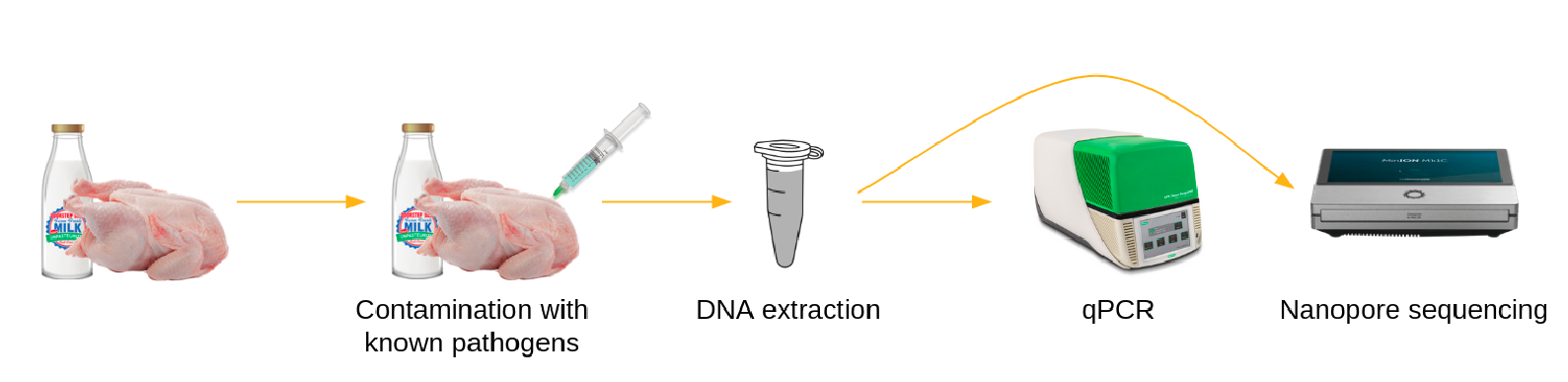
To identify and track foodborne pathogens using long-read metagenomic sequencing, different samples of potentially contaminated food (at different time points or different locations) are prepared, DNA is extracted and sequenced using MinION (ONT). The generated sequencing data then need to be processed using bioinformatics tools.
In this tutorial, we will be presenting a series of Galaxy workflows whose main goals are to:
agnostically detect pathogens (What exactly is this pathogen and what virulence factors does it carry?) from data extracted directly (without prior cultivation) from a potentially contaminated sample (e.g. food like chicken, beef, etc.) and sequenced using Nanopore
compare different samples to trace the possible source of contamination
To illustrate how to process such data, we will use datasets generated by Biolytix with the following approach:
Food samples, here chicken, are spiked with known pathogens, here:
Salmonella enterica subsp. enterica in the sample named Barcode 10 Spike 2
Salmonella enterica subsp. houtenae in the sample named Barcode 11 Spike 2b
DNA in the samples is extracted, analyzed with qPCR, and sequenced via Nanopore. We start the tutorial from raw data generated by Nanopore.
Any analysis should get its own Galaxy history. So let’s start by creating a new one:
Hands On: Data upload
Create a new history for this analysis
To create a new history simply click the new-history icon at the top of the history panel:
Rename the history
Click on galaxy-pencil (Edit) next to the history name (which by default is “Unnamed history”)
Type the new name
Click on Save
To cancel renaming, click the galaxy-undo “Cancel” button
If you do not have the galaxy-pencil (Edit) next to the history name (which can be the case if you are using an older version of Galaxy) do the following:
Click on Unnamed history (or the current name of the history) (Click to rename history) at the top of your history panel
Type the new name
Press Enter
Before we can begin any Galaxy analysis, we need to upload the input data: FASTQ files with the sequenced samples.
Hands On: Import datasets
Import the following samples via link from Zenodo or Galaxy shared data libraries:
Click galaxy-uploadUpload at the top of the activity panel
Select galaxy-wf-editPaste/Fetch Data
Paste the link(s) into the text field
Press Start
Close the window
As an alternative to uploading the data from a URL or your computer, the files may also have been made available from a shared data library:
Go into Libraries (left panel)
Navigate to the correct folder as indicated by your instructor.
On most Galaxies tutorial data will be provided in a folder named GTN - Material –> Topic Name -> Tutorial Name.
Select the desired files
Click on Add to Historygalaxy-dropdown near the top and select as Datasets from the dropdown menu
In the pop-up window, choose
“Select history”: the history you want to import the data to (or create a new one)
Click on Import
Rename the files to Barcode10 and Barcode11 respectively
Click on the galaxy-pencilpencil icon for the dataset to edit its attributes
In the central panel, change the Name field
Click the Save button
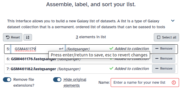
Create a collection named Samples that includes both datasets (Barcode10 and Barcode11)
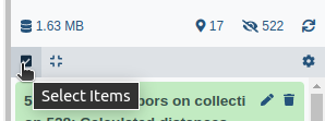
Click on galaxy-selectorSelect Items at the top of the history panel
Check all the datasets in your history you would like to include
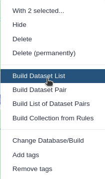
Click n of N selected and choose Advanced Build List
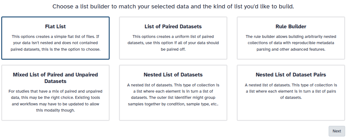
You are in collection building wizard. Choose Flat List and click ‘Next’ button at the right bottom corner.
Double clcik on the file names to edit. For example, remove file extensions or common prefix/suffixes to cleanup the names.
Enter a name for your collection
Click Build to build your collection
Click on the checkmark icon at the top of your history again
In this tutorial, we can offer 2 versions:
A short version, running prebuilt workflows
A long version, going step-by-step
Hands-on: Choose Your Own Tutorial
This is a 'Choose Your Own Tutorial' (CYOT) section (also known as 'Choose Your Own Analysis' (CYOA)), where you can select between multiple paths. Click one of the buttons below to select how you want to follow the tutorial
Preprocessing
Before starting any analysis, it is always a good idea to assess the quality of your input data and to discard poor quality base content by trimming and filtering reads.
In this section we will run a Galaxy workflow that performs the following tasks with the following tools:
We will run all these steps using a single workflow, then discuss each step and the results in more detail.
Hands On: Pre-Processing
Import the workflow into Galaxy
Copy the URL (e.g. via right-click) of this workflow or download it to your computer.
Import the workflow into Galaxy
Click on galaxy-workflows-activityWorkflows in the Galaxy activity bar (on the left side of the screen, or in the top menu bar of older Galaxy instances). You will see a list of all your workflows
Click on galaxy-uploadImport at the top-right of the screen
Provide your workflow
Option 1: Paste the URL of the workflow into the box labelled “Archived Workflow URL”
Option 2: Upload the workflow file in the box labelled “Archived Workflow File”
Click the Import workflow button
Below is a short video demonstrating how to import a workflow from GitHub using this procedure:
Video: Importing a workflow from URL
Run Workflow 1: Nanopore Preprocessingworkflow using the following parameters
“Samples Profile”: PacBio/Oxford Nanopore read to reference mapping, which is the technique used for sequencing the samples.
param-files“Collection of all samples”: Samples collection created from the imported Fastq.qz files
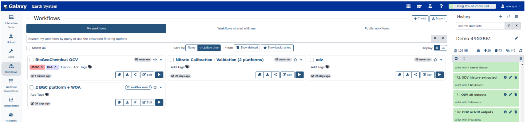
Click on Workflows on the Activity Bar on the left.
At the top of the resulting page you will have the option to switch between the My workflows, Workflows shared with me and Public workflows tabs.
Select the tab you want to see all workflows in that category
Search for your desired workflow.
Click on the workflow name: a pop-up window opens with a preview of the workflow.
To run it directly: click Run (top-right).
Recommended: click Import (left of Run) to make your own local copy under Workflows / My Workflows.
The workflow will take a little while to complete. Once tools have completed, the results will be available in your history for viewing. Note that only the most important outputs will be visible; intermediate files are hidden by default.
While you are waiting for the workflow to complete, please continue reading in the next section(s) where we will go into a bit more detail about what happens at each step of the workflow we launched and examine the results.
Quality Control and Preprocessing
During sequencing, errors are introduced, such as incorrect nucleotides being called. These are due to the technical limitations of each sequencing platform. Sequencing errors might bias the analysis and can lead to a misinterpretation of the data. Sequence quality control is therefore an essential first step in your analysis.
In this tutorial we use similar tools as described in the tutorial “Quality control”, but more specific to Nanopore data:
Quality control with
FastQC generates a web report that will aid you in assessing the quality of your data
NanoPlot plotting tool for long read sequencing data and alignments
Hands On: Initial quality assessment
FastQC ( Galaxy version 0.73+galaxy0) with the following parameters:
param-files“Raw read data from your current history”: Samples collection created from the imported Fastq.qz files
NanoPlot ( Galaxy version 1.28.2+galaxy1) with the following parameters:
“Select multifile mode”: batch
“Type of the file(s) to work on”: fastq
param-files“Data input files”: Samples collection created from the imported Fastq.qz files
Comment
The NanoPlot step, as it does not require the results of FastQC to run, can be launched even if FastQC is not ready
MultiQC ( Galaxy version 1.11+galaxy0) with the following parameters:
In “Results”:
param-repeat“Insert Results”
“Which tool was used generate logs?”: FastQC
In “FastQC output”:
param-repeat“Insert FastQC output”
“Type of FastQC output?”: Raw data
param-files“FastQC output”: collection of Raw data outputs of FastQCtool
Porechop ( Galaxy version 0.2.4) with the following parameters:
param-files“Input FASTA/FASTQ”: Samples collection created from the imported Fastq.qz files
“Output format for the reads”: fastq.gz
fastp ( Galaxy version 0.20.1+galaxy0) with the following parameters:
“Single-end or paired reads”: Single-end
param-files“Input 1”: output collection of Porechoptool
In Output Options
“Output JSON report”: Yes
Comment
This step can be launched even if Porechop is not done. It will be scheduled and wait until Porechop is done to start.
Quality recheck after read trimming and filtering with FastQC and Nanoplot and report aggregation with MultiQC
Hands On: Final quality checks
FastQC ( Galaxy version 0.73+galaxy0) with the following parameters:
param-files“Raw read data from your current history”: output collection of fastptool
NanoPlot ( Galaxy version 1.28.2+galaxy1) with the following parameters:
“Select multifile mode”: batch
“Type of the file(s) to work on”: fastq
param-files“files”: output collection of fastptool
MultiQC ( Galaxy version 1.11+galaxy0) with the following parameters:
In “Results”:
param-repeat“Insert Results”
“Which tool was used generate logs?”: FastQC
In “FastQC output”:
param-repeat“Insert FastQC output”
“Type of FastQC output?”: Raw data
param-files“FastQC output”: collection of Raw data output of FastQCtool done after fastp
param-repeat“Insert Results”
“Which tool was used generate logs?”: fastp
param-files“Output of fastp”: JSON report output of fastptool
Question
Inspect the HTML two outputs of MultiQC for Barcode10 before and after preprocessing tagged MultiQC_Before_Preprocessing and MultiQC_After_Preprocessing
How many sequences does Barcode10 contain before and after trimming?
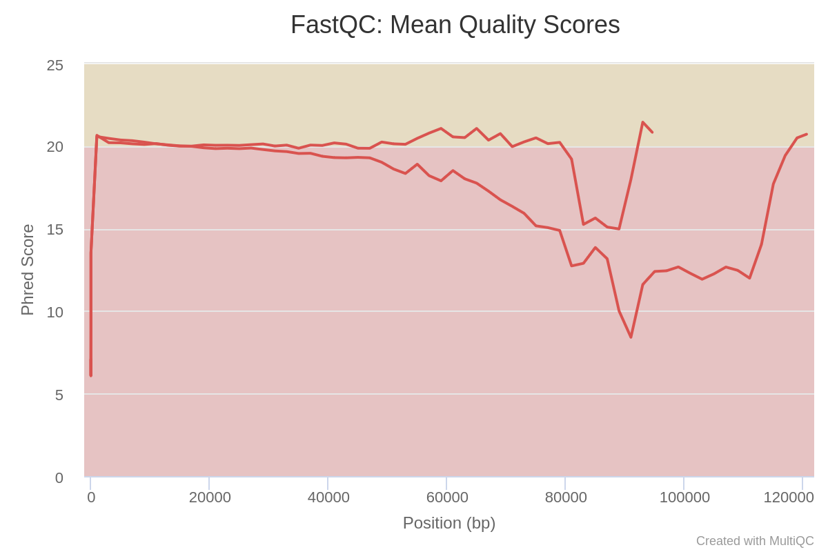
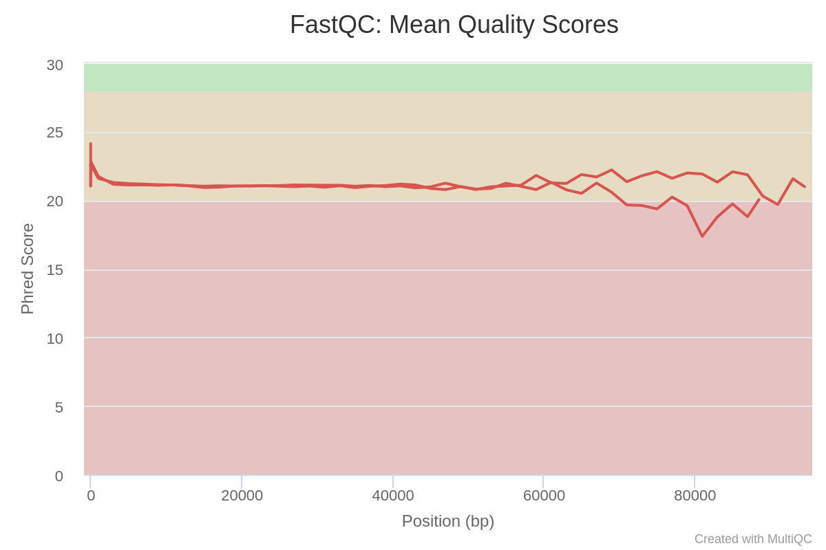
What is the quality score over the reads before and after trimming? And the mean score?
What is the importance of FastQC?
Before trimming the file has 114,986 sequences and After trimming the file has 91,434 sequences
The “Per base sequence quality” is globally medium: the quality score stays above 20 over the entire length of reads after trimming, while quality below 20 could be seen before trimming specially at the beginning and the end of the reads.
Sequence quality of Barcode 10 and Barcode 11 before preprocessing:
Sequence quality of Barcode 10 and Barcode 11 after preprocessing:
After checking what is wrong, e.g. before trimming, we should think about the errors reported by FastQC: they may come from the type of sequencing or what we sequenced (check the “Quality control” training: FastQC for more details). However, despite these challenges, we can already see sequences getting slightly better after the trimming and filtering, so now we can proceed with our analyses.
Comment
For more information about how to interpret the plots generated by FastQC and MultiQC, please see our dedicated “Quality control” Tutorial.
Host read filtering
Generally, we are not interested in the food (host) sequences, rather only those originating from the pathogen itself. It is an important to get rid of all host sequences and to only retain sequences that might include a pathogen, both in order to speed up further steps and to avoid host sequences compromising the analysis.
In this tutorial, we know the samples come from chicken meat spiked with Salmonella so we already know what will we get as the host and the main pathogen. If the host is not known, Kraken2 with Kalamari database can be used to detect it.
In this tutorial we use:
Map reads to chicken reference genome using Map with minimap2 and Chicken (Gallus gallus): galGal6 built in reference genome of chicken, and we move forward with the unmapped ones.
Hands On: Read taxonomic classification for host filtering
Map with minimap2 ( Galaxy version 2.24+galaxy0) with the following parameters:
“Will you select a reference genome from your history or use a built-in index?”: Use a built-in genome index
param-file“Select fastq dataset”: out1 (output of fastptool)
“Select a profile of preset options”: PacBio/Oxford Nanopore read to reference mapping (-Hk19) (map-pb), which is the technique used for sequencing the samples.
In “Alignment options”:
“Customize spliced alignment mode?”: No, use profile setting or leave turned off
Split BAM by reads mapping status ( Galaxy version 2.5.2+galaxy2) with the following parameters:
param-file“BAM dataset to split by mapped/unmapped”: alignment_output (output of Map with minimap2tool)
Samtools fastx ( Galaxy version 1.15.1+galaxy2) with the following parameters:
param-file“BAM or SAM file to convert”: unmapped (output of Split BAM by reads mapping statustool)
“Output format”: compressed FASTQ
“Write index read files”: No
Assign filted reads, after mapping (non chicken reads), to taxa using Kraken2 (Wood and Salzberg 2014) as a further contamination detection using the Kalamari database. The Kalamari database includes mitochondrial sequences of various known hosts including food hosts.
Hands On: Read taxonomic classification for host filtering
Kraken2 ( Galaxy version 2.1.1+galaxy1) with the following parameters:
“Single or paired reads”: Single
param-file“Input sequences”: output (output of Samtools fastxtool)
“Print scientific names instead of just taxids”: Yes
In “Create Report”:
“Print a report with aggregrate counts/clade to file”: Yes
“Report counts for ALL taxa, even if counts are zero”: Yes
“Report minimizer data”: Yes
“Select a Kraken2 database”: kalamari
Question
For the tutorial long version takers, run Samtools fastx on the mapped (output of Split BAM by reads mapping statustool), then inspect the output for Barcode10. If you are a short version taker then inspect the output named host_sequences_fastq.
How many chicken sequences were found?
53722
Filter host assigned reads based on Kraken2 assignments
Manipulate Kraken2 classification to extract the sequence ids of all hosts sequences identified with Kraken2
Filter the FASTQ files to get 1 ouput with the host-assigned sequences and 1 output without the host-assigned reads
Hands On: Host read filtering
Krakentools: Extract Kraken Reads By ID ( Galaxy version 1.2+galaxy1) with the following parameters:
“Single or paired reads?”: Single
param-file“FASTQ/A file”: out1 (output of fastptool)
param-files“Results”: Kraken2 with Kalamri database Results outputs of Kraken2tool
param-files“Report”: Kraken2 with Kalamri database Report outputs of Kraken2tool
“Taxonomix ID(s) to match”:9031 9606 9913
We specify here the taxonomic ID of the hosts so we can filter reads assigned to these hosts. Kraken2 uses taxonomic IDs from NCBI, the IDs for a specific taxa can be found at ncbi. To be generic, we remove here:
Human (9606)
Chicken (9031)
Beef (9913)
If the contaminated food comes from and may include other animals, you can change the value here.
“Invert output”: Yes
“Output as FASTQ”: Yes
“Include parents”: Yes
“Include children”: Yes
Comment
We will need the outputs from this section in the next one. If yours is still running or you get an error you can go on and upload it so you can start the next workflow, the next hands-on is optional.
Hands On: Optional Data upload
Import the quality processed samples fastqsanger files via link from Zenodo or the Shared Data library:
Rename datasets to Barcode10 and Barcode11 respectively
Create a collection named collection of preprocessed samples from the two imported datasets
Taxonomy Profiling
In this section we would like to identify the different organisms found in our samples by assigning taxonomy levels to the reads starting from the kingdom level down to the species level and visualize the result. It’s important to check what might be the species of a possible pathogen to be found, it gets us closer to the investigation as well as discovering possible multiple food infections if any existed.
Taxonomy is the method used to naming, defining (circumscribing) and classifying groups of biological organisms based on shared characteristics such as morphological characteristics, phylogenetic characteristics, DNA data, etc. It is founded on the concept that the similarities descend from a common evolutionary ancestor.
Defined groups of organisms are known as taxa. Taxa are given a taxonomic rank and are aggregated into super groups of higher rank to create a taxonomic hierarchy. The taxonomic hierarchy includes eight levels: Domain, Kingdom, Phylum, Class, Order, Family, Genus and Species.
The classification system begins with 3 domains that encompass all living and extinct forms of life
The Bacteria and Archae are mostly microscopic, but quite widespread.
Domain Eukarya contains more complex organisms
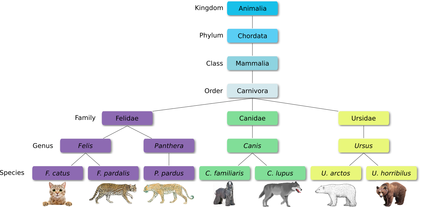
When new species are found, they are assigned into taxa in the taxonomic hierarchy. For example for the cat:
Level
Classification
Domain
Eukaryota
Kingdom
Animalia
Phylum
Chordata
Class
Mammalia
Order
Carnivora
Family
Felidae
Genus
Felis
Species
F. catus
From this classification, one can generate a tree of life, also known as a phylogenetic tree. It is a rooted tree that describes the relationship of all life on earth. At the root sits the “last universal common ancestor” and the three main branches (in taxonomy also called domains) are bacteria, archaea and eukaryotes. Most important for this is the idea that all life on earth is derived from a common ancestor and therefore when comparing two species, you will -sooner or later- find a common ancestor for all of them.
Let’s explore taxonomy in the Tree of Life, using Lifemap
In the previous section we ran Kraken2 along with the Kalamari database, which is also a kind of taxonomy profiling but the database used is designed to include all possible host sequences. In the following part, we run Kraken2 again; but this time with one of its built-in databases, Standard PlusPF, which can give us more insight into pathogen candidate species than Kalamari. You can test this yourself by comparing reports of both Kraken2 runs.
In the \(k\)-mer approach for taxonomy classification, we use a database containing DNA sequences of genomes whose taxonomy we already know. On a computer, the genome sequences are broken into short pieces of length \(k\) (called \(k\)-mers), usually 30bp.
Kraken examines the \(k\)-mers within the query sequence, searches for them in the database, looks for where these are placed within the taxonomy tree inside the database, makes the classification with the most probable position, then maps \(k\)-mers to the lowest common ancestor (LCA) of all genomes known to contain the given \(k\)-mer.
Kraken2 uses a compact hash table, a probabilistic data structure that allows for faster queries and lower memory requirements. It applies a spaced seed mask of s spaces to the minimizer and calculates a compact hash code, which is then used as a search query in its compact hash table; the lowest common ancestor (LCA) taxon associated with the compact hash code is then assigned to the k-mer.
Copy the URL (e.g. via right-click) of this workflow or download it to your computer.
Import the workflow into Galaxy
Run Workflow 2: Taxonomy Profiling and Visualization with Kronaworkflow using the following parameters:
“Send results to a new history”: No
param-files“Collection of preprocessed samples”: collection of preprocessed samples collection, output from Krakentools: Extract Kraken Reads By IDtool from the preproceesing workflow
“Kraken database”: Prebuilt Refseq indexes: PlusPF (Standard plus protozoa and fungi) (Version: 2022-06-07 - Downloaded: 2022-09-04T165121Z)
Click on Workflows on the Activity Bar on the left.
At the top of the resulting page you will have the option to switch between the My workflows, Workflows shared with me and Public workflows tabs.
Select the tab you want to see all workflows in that category
Search for your desired workflow.
Click on the workflow name: a pop-up window opens with a preview of the workflow.
To run it directly: click Run (top-right).
Recommended: click Import (left of Run) to make your own local copy under Workflows / My Workflows.
To assign reads to taxons, we use Kraken2 with Standard PlusPF database.
Hands On: Taxonomy Profiling
Kraken2 ( Galaxy version 2.1.1+galaxy1) with the following parameters:
“Single or paired reads”: Single
param-files“Input sequences”: collection output from Krakentools: Extract Kraken Reads By IDtool from the preprocessing section
In “Create Report”:
“Print a report with aggregrate counts/clade to file”: Yes
“Select a Kraken2 database”: Prebuilt Refseq indexes: PlusPF (Standard plus protozoa and fungi) (Version: 2022-06-07 - Downloaded: 2022-09-04T165121Z)
Question
Inspect the Kraken2 report for Barcode10
What is the most commonly found species?
What is the second most commonly found species?
How many sequences are classified and how many are unclassified?
What are the differences between Kraken2 tool’s report with Kalamari database and Kraken2 tool’s report with Standard PlusPF database regarding the previous 3 questions?
Genus level Salmonella with 9,950 sequences
Genus level Escherichia with 1,949 sequences
33,941 sequences are classified and 3,738 are unclassified
With Kalamari database the most found Genus is Escherichia with 13,943 sequences and the second most found Genus is Salmonella with 10,585 sequences. The number of classified sequences are 30,838 sequences and the unclassified sequences are 6,874. In conclusion, both databases are able to show the similar results of the most common identified species, but with different counts of identified sequences. As well as, the number of the classified sequences with Standard PlusPF database is higher than Kalamari database.
In order to view the taxonomy profiling produced by Kraken2 tool, there are a lot of tools to be used afterwards such as Krona pie chart, which we will be using in this tutorial. For later, you can also check out Pavian tool, as well as Phinch visualization, which is an interactive tool that contains multiple visualization plots, it is interactive alowing you to choose between different parameters, you can visualize each taxonomic level on its own, you can have the metadata of the samples represented along with the taxonomic visualization, download all plots for publications and a lot of other benefits.
Hands On: Visualisation
Krakentools: Convert kraken report file ( Galaxy version 1.2+galaxy1) with the following parameters:
param-file“Kraken report file”: report_output (output of Kraken2tool)
Krona pie chart ( Galaxy version 2.7.1+galaxy0) with the following parameters:
“What is the type of your input data”: Tabular
param-file“Input file”: output (output of Krakentools: Convert kraken report filetool)
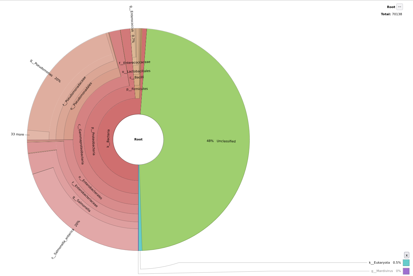
Now let’s explore the Krona pie chart output for Barcode11
Question
What is the most commonly found species?
What is the second most commonly found species?
At Genus level: Salmonella with 16,111 sequences
At Genus level: Pseudomonas with 14,251 sequences
Comment
While these steps are running, you can move on to the next section Gene based pathogenic identification and run the steps there, as well. Both analyses can execute in parallel.
You may have noticed some sequences have been assigned to the Human Genome (Homosapians) species, when we run Kraken2 using the Standard PlusPF in this section. However, in the pre-processing section when we ran Kraken2 with Kalamari no Human Genomes were found. The lab (data producers) has confirmed that these sequences assigned to human by Standard PlusPF database are not human and there should be no human sequences in the samples as Kalamari database result’s confirmed. So these sequences were wrongly assigned to human by Standard PlusPF. That is due to resemblance between organisms and the limited species coverage of Kraken2 databases sometimes do happen that reads corresponding to higher organisms get mapped to humans. It was a very severe problem for the Standard PlusPF, because yeast genes were mis-assigned to human.
We decide to keep these sequences since we do not know what are they via the taxonomy profiling step, which could mean that they might be identified as pathogens in the coming steps, and if we delete them we are possibly losing important information and losing the main goal of the workflow to detect pathogens and track them.
Gene-based pathogen identification
With taxonomy profiling, we identified some bacterial species. But we want to be sure they are pathogenic, by looking for genes known to be linked to pathogenicity or to the pathogenecity character of the organim:
Virulence Factor (VF): gene products, usually proteins, involved in pathogenicity. By identifiying them we can call a pathogen and its severity level
These type of genes have three fundamental mechanisms of antimicrobial resistance that are enzymatic degradation of antibacterial drugs, alteration of bacterial proteins that are antimicrobial targets, and changes in membrane permeability to antibiotics, which will lead to not altering the target site and spread throughput the pathogenic bacteria decreasing the overall fitness of the host.
To look for these genes and determine the strain of the bacteria we are testing for pathogenicity we do:
Generate reports with AMR genes and VF using ABRicate
As outputs, we will get our FASTA and Tabular files to track genes and visualize our pathogenic identification.
Hands On: Gene based Pathogenic Identification
Import the workflow into Galaxy
Copy the URL (e.g. via right-click) of this workflow or download it to your computer.
Import the workflow into Galaxy
Click on galaxy-workflows-activityWorkflows in the Galaxy activity bar (on the left side of the screen, or in the top menu bar of older Galaxy instances). You will see a list of all your workflows
Click on galaxy-uploadImport at the top-right of the screen
Provide your workflow
Option 1: Paste the URL of the workflow into the box labelled “Archived Workflow URL”
Option 2: Upload the workflow file in the box labelled “Archived Workflow File”
Click the Import workflow button
Below is a short video demonstrating how to import a workflow from GitHub using this procedure:
Video: Importing a workflow from URL
Run Workflow 3: Gene-based Pathogen Identificationworkflow using the following parameters:
param-file“Collection of preprocessed samples”: collection of preprocessed samples collection output from Krakentools: Extract Kraken Reads By IDtool from the preprocessing workflow
Click on Workflows on the Activity Bar on the left.
At the top of the resulting page you will have the option to switch between the My workflows, Workflows shared with me and Public workflows tabs.
Select the tab you want to see all workflows in that category
Search for your desired workflow.
Click on the workflow name: a pop-up window opens with a preview of the workflow.
To run it directly: click Run (top-right).
Recommended: click Import (left of Run) to make your own local copy under Workflows / My Workflows.
Assembly
To identify VF or AMR genes, it is better to assemble reads into longer seuqences or contigs, that can be then used to search databases for the presence of any pathogenic gene:
Assembly of long-read metagenomic data using metaflye or Flye.
Hands On: Assembly with Flye
Build list with the following parameters:
In “Dataset”:
param-repeat“Insert Dataset”
param-collection“Input Dataset”: collection output from Krakentools: Extract Kraken Reads By IDtool from the preprocessing section
“Label to use”: Index
Flye ( Galaxy version 2.9+galaxy0) with the following parameters:
param-file“Input reads”: collection output from Build listtool
Comment
We need to run Flye individually on each sample otherwise Flye runs by default a co-assembly mode, i.e. it combines reads of both samples together before running the assembly.
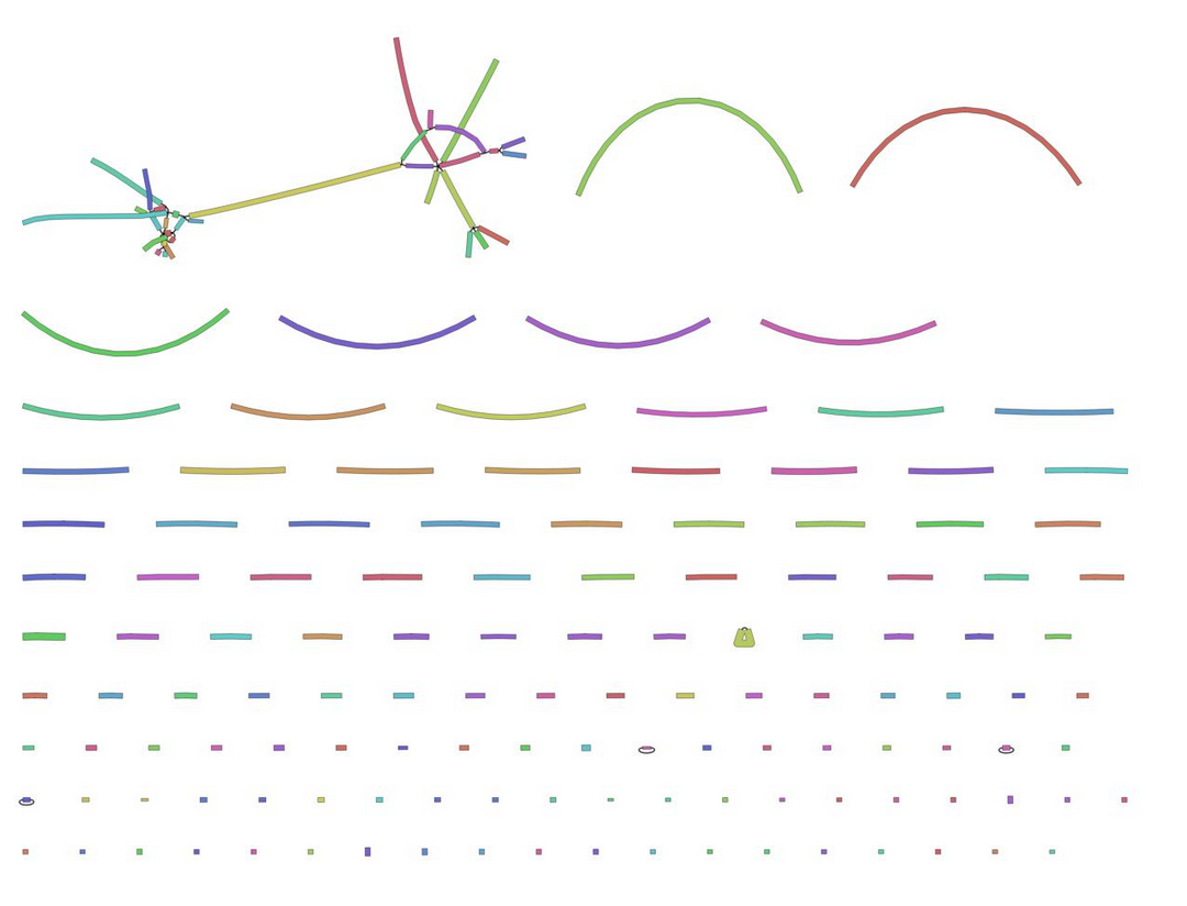
For the visualization of the assembly graph output from Flye we have chosen Bandage Image.
Hands On: Visualization of the assembly grap
Bandage Image ( Galaxy version 0.8.1+galaxy2) with the following parameters:
param-files“Graphical Fragment Assembly”: assembly_graph Assembly graph outputs of Flyetool
Contig polishing using medaka to correct the long, error-prone Nanopore reads
Hands On: Contig polishing
medaka consensus pipeline ( Galaxy version 1.7.2+galaxy0) with the following parameters:
param-files“Select basecalls”: collection output from Krakentools: Extract Kraken Reads By IDtool from the preprocessing section
param-files“Select assembly”: consensus collection output of Flyetool
“Select model”: r941_min_hac_g507
“Select output file(s)”: select all
To keep information about the provenance of the contigs, we extract the sample names from the collection of preprocessed samples collection and add it to the contigs files.
Hands On: Contig renaming to add sample names
FASTA-to-Tabular ( Galaxy version 1.1.1) with the following parameters:
param-files“Convert these sequences”: collection output of medaka consensus pipelinetool
Extract element identifiers ( Galaxy version 0.0.2) with the following parameters:
param-files“Dataset collection”: collection output from Krakentools: Extract Kraken Reads By IDtool from the preprocessing section
Split file ( Galaxy version 0.5.0) with the following parameters:
param-files“Text file to split”: output from Extract element identifierstool
Parse parameter value with the following parameters:
param-files“Input file containing parameter to parse out of”: output from Split filetool
Compose text parameter value ( Galaxy version 0.1.1) with the following parameters:
In “components”:
param-repeat“Insert components”
“Choose the type of parameter for this field”: Text Parameter
“Enter text that should be part of the computed value”: output from Parse parameter valuetool
param-repeat“Insert components”
“Choose the type of parameter for this field”: Text Parameter
“Enter text that should be part of the computed value”: _$1
Replace ( Galaxy version 1.1.4) with the following parameters:
param-file“File to process”: collection output of FASTA-to-Tabulartool
In “Find and Replace”:
param-repeat“Insert Find and Replace”
“Find pattern”: ^(.+)$
“Replace with”: output from Compose text parameter valuetool
“Find-Pattern is a regular expression”: Yes
“Replace all occurences of the pattern”: Yes
“Find and Replace text in”: specific column
“in column”: Column: 1
Tabular-to-FASTA ( Galaxy version 1.1.1) with the following parameters:
param-file“Tab-delimited file”: outfile (output of Replacetool)
“Title column(s)”: c1
“Sequence column”: c2
Rename the output collection Contigs
Question
Inspect Flye and Medaka consensus pipeline output results for Barcode10
How many different contigs did you get after Flye, collection name: Flye Consensus Fasta?
How many were left after Medaka consensus pipeline, collection name: Sample all contigs, and what does that mean?
What is the result of your Bandage Image?
After Flye we have got 130 contigs
After Medaka consensus pipeline all 130 contigs were kept, which means that the quality of the Flye run was high, and as a result the polishing did not remove any of the contigs.
The graph looks like:
Antimicrobial Resistance Genes
Now, to search AMR genes among our samples’ contigs, we run ABRicate and choose the NCBI Bacterial Antimicrobial Resistance Gene Database (AMRFinderPlus) from the advanced options of the tool. The tool checks if there is an AMR found or not, if found then in which contig it is, its location on the contig, what the name of the exact product is, what substance it provides resistance against and a lot of other information regarding the found AMR.
Hands On: Antimicrobial Resistance Genes Identification
ABRicate ( Galaxy version 1.0.1) with the following parameters:
param-files“Input file (Fasta, Genbank or EMBL file)”: collection output of medaka consensus pipelinetool FASTA files with contigs
In “Advanced options”:
“Database to use - default is ‘resfinder’“: NCBI Bacterial Antimicrobial Resistance Reference Gene Database
Rename ABRicate the output collection amr_identified_by_ncbi
The outputs of ABRicate is a tabular file with different columns:
FILE: The filename this hit came from
SEQUENCE: The sequence in the filename
START: Start coordinate in the sequence
END: End coordinate
STRAND: AMR gene
GENE: AMR gene
COVERAGE: What proportion of the gene is in our sequence
COVERAGE_MA: A visual represenation
GAPS: Was there any gaps in the alignment - possible pseudogene?
%COVERAGE: Proportion of gene covered
%IDENTITY: Proportion of exact nucleotide matches
DATABASE: The database this sequence comes from
ACCESSION: The genomic source of the sequence
PRODUCT
RESISTANCE
To prepare the ABRicatetool output tabulars of both samples for further analysis in the Pathogen Detection Samples Aggregation and Visualisation section, tabular manipulation tools such as Replacetool is used. We mainly use it to add the sample ID along with which contig at which exact location.
Hands On: Antimicrobial Resistance Genes Identification
Replace ( Galaxy version 1.1.4) with the following parameters:
param-file“File to process”: report (output of ABRicatetool)
In “Find and Replace”:
param-repeat“Insert Find and Replace”
“Find pattern”: #FILE
“Replace with”: SampleID
“Replace all occurences of the pattern”: Yes
“Find and Replace text in”: specific column
“in column”: c1
param-repeat“Insert Find and Replace”
“Find pattern”: ^(.+)$
“Replace with”: output from Compose text parameter valuetool
“Find-Pattern is a regular expression”: Yes
“Replace all occurences of the pattern”: Yes
“Ignore first line”: Yes
“Find and Replace text in”: specific column
“in column”: c2
Rename the output collection AMRs
Question
Inspect ABRicate output files from Barcode10and Barcode11 tags
How many AMR genes found in Barcode10 sample, what are they? Give more details about them.
How many AMR genes found in Barcode11 sample, what are they? Give more details about them.
7 AMR genes were found:
Tet(C), which resists TETRACYCLINE. It was found in contig 119 from the position 1635 till 2810, with 100% coverage, so 100% of gene is covered in this contig.
Tet(34), which resists TETRACYCLINE. It was found in contig 135 from the position 69874 till 70223, with 74.41% coverage.
aac(6’)_Yersi, which resists AMINOGLYCOSIDE. It was found in contig 156 from the position 37698 till 38000, with 69.68 % coverage.
2 genes with sulfonamide-resistant dihydropteroate synthase Sul1 products
2 genes with oxacillin-hydrolyzing class D beta-lactamase OXA-2 products
2 AMR genes were found by the database in Barcode11 sample, Tet(34) and aac(6’)_Yersi.
Virulence Factor identification
In this step we return back to the main goal of the tutorial where we want to identify the pathogens: identify if the bacteria found in our samples are pathogenic bacteria or not. One of the ways to do that is to identify if the sequences include genes with a Virulence Facor or not, such that if the samples include gene(s) with a Virulence Factor then it for sure is a pathogen.
Comment: Definitions
Bacterial Pathogen: A bacterial pathogen is usually defined as any bacterium that has the capacity to cause disease. Its ability to cause disease is called pathogenicity.
Virulence: Virulence provides a quantitative measure of the pathogenicity or the likelihood of causing a disease.
Virulence Factors: Virulence factors refer to the properties (i.e., gene products) that enable a microorganism to establish itself on or within a host of a particular species and enhance its potential to cause disease. Virulence factors include bacterial toxins, cell surface proteins that mediate bacterial attachment, cell surface carbohydrates and proteins that protect a bacterium, and hydrolytic enzymes that may contribute to the pathogenicity of the bacterium.
To identifly VFs, we use again ABRicate but this time with the VFDB from the advanced options of the tool.
Hands On: Virulence Factor identification
ABRicate ( Galaxy version 1.0.1) with the following parameters:
param-files“Input file (Fasta, Genbank or EMBL file)”: collection output of medaka consensus pipelinetool FASTA files with contigs
In “Advanced options”:
“Database to use - default is ‘resfinder’“: VFDB
Rename ABRicate the output collection vfs_of_genes_identified_by_vfdb
Question
Inspect VFs of genes Identified by VFDB output file fromBarcode10and Barcode11
How many different VFs gene products were found in Barcode10 sample?
How many different VFs gene products were found in Barcode11 sample?
188
287
To prepare the ABRicatetool output tabulars of both samples for further analysis in the Pathogen Detection Samples Aggregation and Visualisation section, tabular manipulation tools such as Replacetool is used. We mainly use it to add the sample ID along with which contig at which exact location.
Hands On: Replace Text
Replace ( Galaxy version 1.1.4) with the following parameters:
param-file“File to process”: report (output of ABRicatetool)
In “Find and Replace”:
param-repeat“Insert Find and Replace”
“Find pattern”: #FILE
“Replace with”: SampleID
“Replace all occurences of the pattern”: Yes
“Find and Replace text in”: specific column
“in column”: c1
param-repeat“Insert Find and Replace”
“Find pattern”: ^(.+)$
“Replace with”: output from Compose text parameter valuetool
“Find-Pattern is a regular expression”: Yes
“Replace all occurences of the pattern”: Yes
“Ignore first line”: Yes
“Find and Replace text in”: specific column
“in column”: c2
Rename the output collection VFs
Allele-based pathogen identification
Now we would like to identify pathogens with a third approach based on variant and single nucleotide polymorphisms (SNPs) calling: comparison of reads to a targeted reference genome, and call the differences between sample reads and reference genomes to identify variants.
For example, if we want to check whether our samples include Campylobacter pathogenic strains or not, we will map our samples against the reference genome of the Campylobacter species. Variants in specific positions on the genome are queried to judge if these variations would indicate a pathogen or not.
This approach also allows identification of novel alleles and possible new variants of the pathogen.
Using this approach, we also build the consensus genome of each sample, so we can later build a phylogenetic tree of all samples’ full genomes and have an insight into events that occurred during the evolution of same or different species in the samples.
Copy the URL (e.g. via right-click) of this workflow or download it to your computer.
Import the workflow into Galaxy
Click on galaxy-workflows-activityWorkflows in the Galaxy activity bar (on the left side of the screen, or in the top menu bar of older Galaxy instances). You will see a list of all your workflows
Click on galaxy-uploadImport at the top-right of the screen
Provide your workflow
Option 1: Paste the URL of the workflow into the box labelled “Archived Workflow URL”
Option 2: Upload the workflow file in the box labelled “Archived Workflow File”
Click the Import workflow button
Below is a short video demonstrating how to import a workflow from GitHub using this procedure:
Video: Importing a workflow from URL
Run Workflow 4: Nanopore Allele-based Pathogen Identificationworkflow using the following parameters:
“Send results to a new history”: No
param-files“Collection of preprocessed samples”: collection of preprocessed samples collection output from Krakentools: Extract Kraken Reads By IDtool from the preprocessing workflow
“Samples Profile”: Nothing selected
Samples profile is the technique used for sequencing the samples, it is an optional input, if you choose nothing, the tool will automatically detect it based on the input samples reads.
param-file“Reference Genome of Tested Strain”: Salmonella_Ref_genome.fna.gz
Variant Calling or SNP Calling
To identify variants, we
Map reads to the reference genome of the species of the pathogen we want to test our samples against using Minimap2 (Li 2017) as our datasets are from a Nanopore:
Hands On: Mapping to reference genome
Map with minimap2 ( Galaxy version 2.24+galaxy0) with the following parameters:
“Will you select a reference genome from your history or use a built-in index?”: Use a genome from history and build index
param-file“Use the following dataset as the reference sequence”: Salmonella_Ref_genome.fna.gz
“Single or Paired-end reads”: Single
param-files“Select fastq dataset”: collection output from Krakentools: Extract Kraken Reads By IDtool from the preprocessing section
Identify variants and single nucleotide variants using Clair3 (Zheng et al. 2021), which is designed specifically for Nanopore datasets and giving better results than other variant calling tools, as well as being new and up-to-date.
The output is a VCF file. VCF is the standard file format for storing variation data, with different columns:
#CHROM: Chromosome
POS: Co-ordinate - The start coordinate of the variant.
ID: Identifier
REF: Reference allele - The reference allele is whatever is found in the reference genome. It is not necessarily the major allele.
ALT: Alternative allele - The alternative allele is the allele found in the sample you are studying.
QUAL: Score - Quality score out of 100.
FILTER: Pass/fail - If it passed quality filters.
INFO: Further information - Allows you to provide further information on the variants. Keys in the INFO field can be defined in header lines above thetable.
FORMAT: Information about the following columns - The GT in the FORMAT column tells us to expect genotypes in the following columns.
Individual identifier (optional) - The previous column told us to expect to see genotypes here. The genotype is in the form “0|1”, where 0 indicates the reference allele and 1 indicates the alternative allele, i.e it is heterozygous. The vertical pipe “|” indicates that the genotype is phased, and is used to indicate which chromosome the alleles are on. If this is a slash (/) rather than a vertical pipe, it means we don’t know which chromosome they are on.
Extract a tabular report with Chromosome, Position, Identifier, Reference allele, Alternative allele and Filter from the VCF files using SnpSift Extract Fields
Hands On: Extract a tabular report
SnpSift Extract Fields ( Galaxy version 4.3+t.galaxy0) with the following parameters:
param-files“Variant input file in VCF format”: collection output of SnpSift Filter
“Fields to extract”: CHROM POS ID REF ALT FILTER
Question
Now let’s inspect the outputs for Barcode10:
How many variants were found by Clair3?
How many variants were found after quality filtering?
Before filtering: 2,812
After filtering 2,642
Mapping Depth and Coverage
Mapping depth and coverage are essential metrics in variant calling because they ensure comprehensive analysis and accuracy in genomic studies. Mapping coverage indicates the percentage of the reference genome covered by sequencing reads, ensuring that the majority of the genome is analyzed to detect variants accurately. Mapping depth, on the other hand, refers to the number of times each base is sequenced, providing confidence in variant calls by distinguishing true variants from sequencing errors and enabling the detection of low-frequency variants. Both metrics are crucial for quality control, resource allocation, and reliable interpretation of genomic data, ensuring that important variants are not missed and reducing the risk of false positives or negatives.
Samtools depth ( Galaxy version 1.15.1+galaxy2) with the following parameters:
param-file“BAM file(s)”: alignment_output (output of Map with minimap2tool)
“Filter by regions”: No
Samtools coverage ( Galaxy version 1.15.1+galaxy2) with the following parameters:
“Are you pooling bam files?”: No
param-file“BAM file”: alignment_output (output of Map with minimap2tool)
“Histogram”: No
Question
Inspect the Samtools coverage output for Barcode10
How well the sample reads covering the reference genome of Salmonella?
99.65%.
Consensus Genome Building
For further anaylsis we have included one more step in this section, where we build the full genome of our samples.
This consensus genome can be used later to compare and relate samples together based on their full genome. In cases such as SARS-CoV2, it is important to do so in order to discover new outbreaks. In this example of the training, it is not really important to draw a tree of the full genomes of the samples as Salmonella does not have such a speedy outbreak as SARS-CoV2 does. However, we decided to include it in the workflow for any further analysis of the users, if needed.
Inspect the bcftools consensus output for Barcode11
How many sequences did we get for the sample? What are they?
Why?
We got 2 sequences: the complete genome and the complete plasmid genome.
The tool uses the reference genome and the variants found to build the consensus genome of the sample, and the reference genome FASTA file we use includes two sequences a complete one and a plasmid complete one. So the tool constructed both sequences for us to choose from, based on our further analysis.
Pathogen Detection Samples Aggregation and Visualisation
Comment
If you did not get your Gene-based pathogen identification section output files needed yet or you got an error for some reason, you can go on and download them all or the ones missing from Zenodo so you can start this workflow, please don’t forget to create the collections for them as explained in the pervious hands-on.
Hands On: Optional Data upload
Import all tabular and FASTA files needed for this section via link from Zenodo to the new created history:
Click galaxy-uploadUpload at the top of the activity panel
Select galaxy-wf-editPaste/Fetch Data
Paste the link(s) into the text field
Press Start
Close the window
In this last section, we would like to show how to aggregate results and use the results to help tracking pathogenes among samples by:
Drawing a presence-absence heatmap of the identified VF genes within all samples to visualize in which samples these genes can be found.
Drawing a phylogenetic tree for each pathogenic gene detected, where we will relate the contigs of the samples together where this gene is found.
With these two types of visualizations we can have an overview of all samples and the genes, but also how samples are related to each other i.e. which common pathogenic genes they share. Given the time of the sampling and the location one can easily identify using these graphs, where and when the contamination has occurred among the different samples.
Hands On: Organize imported data
Follow these steps only if you imported the datasets, but if your Gene-based Pathogen Identification part is already finished correctly then skip the following 3 steps.
Create a collection named VFs with VFs files
Click on galaxy-selectorSelect Items at the top of the history panel
Check all the datasets in your history you would like to include
Click n of N selected and choose Advanced Build List
You are in collection building wizard. Choose Flat List and click ‘Next’ button at the right bottom corner.
Double clcik on the file names to edit. For example, remove file extensions or common prefix/suffixes to cleanup the names.
Enter a name for your collection
Click Build to build your collection
Click on the checkmark icon at the top of your history again
Create a collection named vfs_of_genes_identified_by_vfdb with vfs_of_genes_identified_by_vfdb files
Create a collection named Contigs with Contigs files
Comment
If you did not get your Gene-based pathogen identification section output files needed yet or you got an error for some reason, you can go on and download them all or the ones missing from Zenodo so you can start this workflow, please don’t forget to create the collections for them as explained in the pervious hands-on. You also need to download and import more tabular files that are generated from the output of Preprocessing and Allele-based pathogen identification.
Hands On: Optional Data upload
Import all tabular and FASTA files needed for this section via link from Zenodo to the new created history:
Click galaxy-uploadUpload at the top of the activity panel
Select galaxy-wf-editPaste/Fetch Data
Paste the link(s) into the text field
Press Start
Close the window
In this last section, we would like to show how to aggregate results and use the results to help tracking pathogenes among samples by:
Drawing a presence-absence heatmap of the identified VF genes within all samples to visualize in which samples these genes can be found.
Drawing a phylogenetic tree for each pathogenic gene detected, where we will relate the contigs of the samples together where this gene is found.
With the visualizations types in this workflow, e.g. Heatmaps, Phylogenetic trees and Barplots, we can have an overview of all samples and the genes, but also how samples are related to each other i.e. which common pathogenic genes they share. Given the time of the sampling and the location one can easily identify using these graphs, where and when the contamination has occurred among the different samples.
Hands On: Organize imported data
Follow these steps only if you imported the datasets, but if your Gene-based Pathogen Identification part is already finished correctly then skip the following 5 steps.
Create a collection named VFs with VFs files
Click on galaxy-selectorSelect Items at the top of the history panel
Check all the datasets in your history you would like to include
Click n of N selected and choose Advanced Build List
You are in collection building wizard. Choose Flat List and click ‘Next’ button at the right bottom corner.
Double clcik on the file names to edit. For example, remove file extensions or common prefix/suffixes to cleanup the names.
Enter a name for your collection
Click Build to build your collection
Click on the checkmark icon at the top of your history again
Create a collection named vfs_of_genes_identified_by_vfdb with vfs_of_genes_identified_by_vfdb files
Create a collection named AMRs with AMRs files
Create a collection named amr_identified_by_ncbi with amr_identified_by_ncbi files
Create a collection named Contigs with Contigs files
Hands On: All Samples Analysis
Import the workflow into Galaxy
Copy the URL (e.g. via right-click) of this workflow or download it to your computer.
Import the workflow into Galaxy
Click on galaxy-workflows-activityWorkflows in the Galaxy activity bar (on the left side of the screen, or in the top menu bar of older Galaxy instances). You will see a list of all your workflows
Click on galaxy-uploadImport at the top-right of the screen
Provide your workflow
Option 1: Paste the URL of the workflow into the box labelled “Archived Workflow URL”
Option 2: Upload the workflow file in the box labelled “Archived Workflow File”
Click the Import workflow button
Below is a short video demonstrating how to import a workflow from GitHub using this procedure:
Video: Importing a workflow from URL
Run Workflow 5: Pathogen Detection Samples Aggregation and Visualisationworkflow using the following parameters:
“Send results to a new history”: No
param-collection“Contigs”: collection Contigs output from the Gene-based Pathogen Identification workflow
param-collection“VFs”: collection VFs output from the Gene-based Pathogen Identification workflow
param-collection“AMRs”: collection AMRs output from the Gene-based Pathogen Identification workflow
param-collection“vfs_of_genes_identified_by_vfdb”: collection vfs_of_genes_identified_by_vfdb output from the Gene-based Pathogen Identification workflow
param-collection“amr_identified_by_ncbi”: collection amr_identified_by_ncbi output from the Gene-based Pathogen Identification workflow
param-collection“removed_hosts_percentage_tabular”: tabular removed_hosts_percentage_tabular output from the Preprocessing workflow
param-collection“mapping_coverage_percentage_per_sample”: tabular mapping_coverage_percentage_per_sample output from the Allele-based Pathogen Identification workflow
param-collection“mapping_mean_depth_per_sample”: tabular mapping_mean_depth_per_sample output from the Allele-based Pathogen Identification workflow
param-collection“number_of_variants_per_sample”: tabular number_of_variants_per_sample output from the Allele-based Pathogen Identification workflow
Click on Workflows on the Activity Bar on the left.
At the top of the resulting page you will have the option to switch between the My workflows, Workflows shared with me and Public workflows tabs.
Select the tab you want to see all workflows in that category
Search for your desired workflow.
Click on the workflow name: a pop-up window opens with a preview of the workflow.
To run it directly: click Run (top-right).
Recommended: click Import (left of Run) to make your own local copy under Workflows / My Workflows.
Heatmap
A heatmap is one of the visualization techniques that can give you a complete overview of all the samples together and whether or not a certain value exists. In this tutorial, we use the heatmap to visualize all samples aside and check which common bacteria pathogen genes are found in samples and which is only found in one of them.
We use Heatmap w ggplot tool along with other tabular manipulating tools to prepare the tabular files.
Combine VFs accessions for samples into a table and get 0 or 1 for absence / presence
Hands On: Heatmap
Remove beginning with the following parameters:
param-collection“from”: vfs_of_genes_identified_by_vfdb collection output of ABRicatetool from the Gene-based Pathogen Identification section
Group with the following parameters:
param-file“Select data”: out_file1 (output of Remove beginningtool)
“Group by column”: c6
In “Operation”:
param-repeat“Insert Operation”
“Type”: Count
“On column”: c6
Filter empty datasets with the following parameters:
param-file“Input Collection”: out_file1 (output of Grouptool)
Column join ( Galaxy version 0.0.3) with the following parameters:
param-file“Tabular files”: output (output of Filter empty datasetstool)
“Fill character”: 0
Column Regex Find And Replace ( Galaxy version 1.0.3) with the following parameters:
param-file“Select cells from”: tabular_output (output of Column jointool)
“using column”: c1
In “Check”:
param-repeat“Insert Check”
“Find Regex”: #KEY
“Replacement”: key
Draw heatmap
Hands On: Heatmap
Heatmap w ggplot ( Galaxy version 3.4.0+galaxy0) with the following parameters:
param-file“Select table”: out_file1 (output of Column Regex Find And Replacetool)
“Select input dataset options”: Dataset with header and row names
“Select column, for row names”: c1
“Sample names orientation”: vertial
“Plot title”: Pathogeneic Genes Per Samples
In “Advanced Options”:
“Enable data clustering”: Yes
In “Output Options”:
“Unit of output dimensions”: Centimeters (cm)
“width of output”: 70.0
“height of output”: 70.0
“dpi of output”: 1000.0
“Additional output format”: PDF
Question
Now let’s see how your heatmap PDF looks like, you can zoom-in and out in your Galaxy history.
Mention three of the common bacterial pathogen genes found in both samples.
How can the differences in the found VF bacteria pathogen genes between the two samples be interpreted?
A lot of bacteria pathogen VF gene products identified by the VFDB are common in both samples, such as: rfaD, ssaN and fliQ
Both samples were spiked with the same pathogen species, S. enterica, but not the same strain:
Barcode10 sample is spiked with S. enterica subsp. enterica strain
Barcode11 sample is spiked with S. enterica subsp. houtenae strain.
This can be the main cause of the big similarities and the few differences of the bacteria pathogen VF gene products found between both of the two samples.
Other factors such as the time and location of the sampling may cause other differences. By knowing the metadata of the samples inputted for the workflows in real life we can understand what actually happened. We can have samples with no pathogen found then we start detecting genes from the 7th or 8th sample, then we can identify where and when the pathogen entered the host, and stop the cause of that
Phylogenetic Tree building
Phylogenetic trees can be used to track the evolution of the pathogen between the samples. Therefore, the VFs are used as a marker gene for the pathogen, similar to 16S marker genes for species profiling. We use the VFs since we know they are associated to the pathogenicity of the sample. By observing the created trees one can identify groups of related pathogens. If additional meta data of the samples would be available one could further identify groups that are associated to specific traits such as increase pathogenicity or faster transmission. Consequently, the tree could be used for phylogenetic placement of unknwon samples.
For the phylogenetic trees, for each bacteria pathogen gene found in the samples we use ClustalW (Larkin et al. 2007) for Multiple Sequence Alignment (MSA) needed before constructing a phylogenetic tree, for the tree itself we use FASTTREE and Newick Display (Dress et al. 2008) to visualize it.
To get the sequence to align, we need to extract the sequences of the VFs in the contigs:
Hands On: Extract the sequences of the VFs
Collapse Collection ( Galaxy version 5.1.0) with the following parameters:
param-collection“Collection of files to collapse into single dataset”: Contigs
“Prepend File name”: Yes
Collapse Collection ( Galaxy version 5.1.0) with the following parameters:
param-collection“Collection of files to collapse into single dataset”: VFs
“Keep one header line”: Yes
“Prepend File name”: Yes
Split by group ( Galaxy version 0.6) with the following parameters:
param-file“File to split”: output of 2nd Collapse Collectiontool
“on column”: Column: 13
“Include header in splits?”: Yes
Cut with the following parameters:
“Cut columns”: c2,c3,c4
param-file“From”: split_output (output of Split by grouptool)
Remove beginning with the following parameters:
param-file“from”: output of Cuttool
bedtools getfasta ( Galaxy version 2.30.0+galaxy1) with the following parameters:
param-file“BED/bedGraph/GFF/VCF/EncodePeak file”: out_file1 (output of Remove beginningtool)
“Choose the source for the FASTA file”: History
param-file“FASTA file”: output (output of 1st Collapse Collectiontool)
We can now run multiple sequence alignment, build the trees for each VF and display them.
Hands On: Phylogenetic Tree building
ClustalW ( Galaxy version 2.1+galaxy1) with the following parameters:
param-collection“FASTA file”: output of bedtools getfastatool
“Data type”: DNA nucleotide sequences
“Output alignment format”: FASTA format
“Output complete alignment (or specify part to output)”: Complete alignment
FASTTREE ( Galaxy version 2.1.10+galaxy1) with the following parameters:
“Aligned sequences file (FASTA or Phylip format)”: fasta
param-collection“FASTA file”: output of ClustalWtool
“Set starting tree(s)”: No starting trees
“Protein or nucleotide alignment”: Nucleotide
Newick Display ( Galaxy version 1.6+galaxy1) with the following parameters:
param-file“Newick file”: output of FASTTREEtool
“Branch support”: Hide branch support
“Branch length”: Hide branch length
“Image width”: 2000
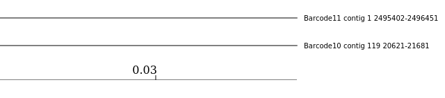
Question
Now let’s see how your trees for the bacteria pathogen gene with accession IDs: AAF37887 and NP_459543 look like. To access that go to the output of Newick
In which samples and contigs is gene AAF37887 found?
In which samples and contigs is gene NP_459543 found?
In the Barcode10: Contig 149 and Barcode11: Contig 4
In the Barcode10: Contig 91 and Barcode11: Contig 4
Conclusion
In this tutorial, we have tried the workflow designed to detect and track pathogens in our food and drinks. Through out the full workflow we used our Nanopore sequenced datasets from Biolytix and analyzed it, found the pathogens and tracked it. This approach can be summarized with the following scheme:
Figure 1: The complete picture of the workflow used in this training highlighting, not all, but the most important steps done in 5 sub-workflows explained in the training
You've Finished the Tutorial
Please also consider filling out the Feedback Form as well!
Frequently Asked Questions
Have questions about this tutorial? Have a look at the available FAQ pages and support channels
Further information, including links to documentation and original publications, regarding the tools, analysis techniques and the interpretation of results described in this tutorial can be found here.
References
Larkin, M. A., G. Blackshields, N. P. Brown, R. Chenna, P. A. McGettigan et al., 2007 Clustal W and Clustal X version 2.0. Bioinformatics 23: 2947–2948. 10.1093/bioinformatics/btm404
Dress, A. W. M., C. Flamm, G. Fritzsch, S. Gr\~ A1\textfractionsolidus4newald, M. Kruspe et al., 2008 Noisy: Identification of problematic columns in multiple sequence alignments. Algorithms for Molecular Biology 3: 7. 10.1186/1748-7188-3-7
Li, H., B. Handsaker, A. Wysoker, T. Fennell, J. Ruan et al., 2009 The Sequence Alignment/Map format and SAMtools. Bioinformatics 25: 2078–2079. 10.1093/bioinformatics/btp352
Cingolani, P., V. M. Patel, M. Coon, T. Nguyen, S. J. Land et al., 2012 Using Drosophila melanogaster as a Model for Genotoxic Chemical Mutational Studies with a New Program, SnpSift. Frontiers in Genetics 3: 10.3389/fgene.2012.00035
Wood, D. E., and S. L. Salzberg, 2014 Kraken: ultrafast metagenomic sequence classification using exact alignments. Genome Biology 15: R46. 10.1186/gb-2014-15-3-r46
Wick, R. R., M. B. Schultz, J. Zobel, and K. E. Holt, 2015 Bandage: interactive visualization of \lessi\greaterde novo\less/i\greater genome assemblies. Bioinformatics 31: 3350–3352. 10.1093/bioinformatics/btv383
Ewels, P., M. Magnusson, M. Käller, and S. Lundin, 2016 MultiQC: summarize analysis results for multiple tools and samples in a single report. Bioinformatics 32: 3047–3048. 10.1093/bioinformatics/btw354
Li, H., 2017 Minimap2: fast pairwise alignment for long nucleotide sequences. https://arxiv.org/abs/1708.01492. 10.1093/bioinformatics/bty191
Chen, S., Y. Zhou, Y. Chen, and J. Gu, 2018 fastp: an ultra-fast all-in-one FASTQ preprocessor. 10.1093/bioinformatics/bty560
Kolmogorov, M., D. Bickhart, B. Behsaz, A. Gurevich, M. Rayko et al., 2020 metaFlye: scalable long-read metagenome assembly using repeat graphs. Nature Methods 17: 1–8. 10.1038/s41592-020-00971-x
Zheng, Z., S. Li, J. Su, A. W.-S. Leung, T.-W. Lam et al., 2021 Symphonizing pileup and full-alignment for deep learning-based long-read variant calling. 10.1038/s43588-022-00387-x
Feedback
Did you use this material as an instructor? Feel free to give us feedback on how it went.
Did you use this material as a learner or student? Click the form below to leave feedback.
Hiltemann, Saskia, Rasche, Helena et al., 2023 Galaxy Training: A Powerful Framework for Teaching! PLOS Computational Biology 10.1371/journal.pcbi.1010752
Batut et al., 2018 Community-Driven Data Analysis Training for Biology Cell Systems 10.1016/j.cels.2018.05.012
@misc{microbiome-pathogen-detection-from-nanopore-foodborne-data,
author = "Bérénice Batut and Engy Nasr and Paul Zierep",
	title = "Pathogen detection from (direct Nanopore) sequencing data using Galaxy - Foodborne Edition (Galaxy Training Materials)",
	year = "",
	month = "",
	day = "",
	url = "\url{https://training.galaxyproject.org/training-material/topics/microbiome/tutorials/pathogen-detection-from-nanopore-foodborne-data/tutorial.html}",
	note = "[Online; accessed TODAY]"
}
@article{Hiltemann_2023,
	doi = {10.1371/journal.pcbi.1010752},
	url = {https://doi.org/10.1371%2Fjournal.pcbi.1010752},
	year = 2023,
	month = {jan},
	publisher = {Public Library of Science ({PLoS})},
	volume = {19},
	number = {1},
	pages = {e1010752},
	author = {Saskia Hiltemann and Helena Rasche and Simon Gladman and Hans-Rudolf Hotz and Delphine Larivi{\`{e}}re and Daniel Blankenberg and Pratik D. Jagtap and Thomas Wollmann and Anthony Bretaudeau and Nadia Gou{\'{e}} and Timothy J. Griffin and Coline Royaux and Yvan Le Bras and Subina Mehta and Anna Syme and Frederik Coppens and Bert Droesbeke and Nicola Soranzo and Wendi Bacon and Fotis Psomopoulos and Crist{\'{o}}bal Gallardo-Alba and John Davis and Melanie Christine Föll and Matthias Fahrner and Maria A. Doyle and Beatriz Serrano-Solano and Anne Claire Fouilloux and Peter van Heusden and Wolfgang Maier and Dave Clements and Florian Heyl and Björn Grüning and B{\'{e}}r{\'{e}}nice Batut and},
	editor = {Francis Ouellette},
	title = {Galaxy Training: A powerful framework for teaching!},
	journal = {PLoS Comput Biol}
}
Funding
These individuals or organisations provided funding support for the development of this resource
5 stars:
Liked: Engy Nasr you're SO good at explaining ! I'm a beginner in bioinformatics, just started a master's on the topic and I was struggling to understand the procedures that's why I joined the Galaxy training, you made it SO easy to follow, thank you very much seriously I'm so excited to starr using what you've taught, I work in AMR research so this is going to be very helpful, such a lifesaver. ´ THANKS!
Disliked: I like everything, my favorite tutorial so far.
May 2023
5 stars:
Liked: Good overview of the tools used and why they were used.
Questions:
")


 of the genomes that contain that k-mer in the database. The taxa associated with the sequence's k-mers, as well as the taxa's ancestors, form a pruned subtree of the general taxonomy tree, which is used for classification. In the classification tree, each node has a weight equal to the number of k-mers in the sequence associated with the node's taxon. Each root-to-leaf (RTL) path in the classification tree is scored by adding all weights in the path, and the maximal RTL path in the classification tree is the classification path (nodes highlighted in yellow). The leaf of this classification path (the orange, leftmost leaf in the classification tree) is the classification used for the query sequence. Source: <span class=\"citation\"><a href=\"#Wood2014\">Wood and Salzberg 2014</a></span>")

 Open image in new tab