In many organism, transcription factors (TF) play an important tole in the regulation of the gene expression. In human, we have up to 2,800 proteins and more than 1,600 are
TF (list of transcription factors), although the number might change over timer.
Investigating the role of TFs, such as GATA1, is a very important task to understand the regulatory mechanisms in the cell and thus ascertain
the source of a disease, such as myelofibrosis a type of blood cancer.
Cleavage Under Targets and Release Using Nuclease (CUT&RUN) Skene and Henikoff 2017 became the new and advanced method to analyse DNA-associated proteins. CUT&RUN uses an antibody just as ChIP-Seq to select the protein of interest (POI).
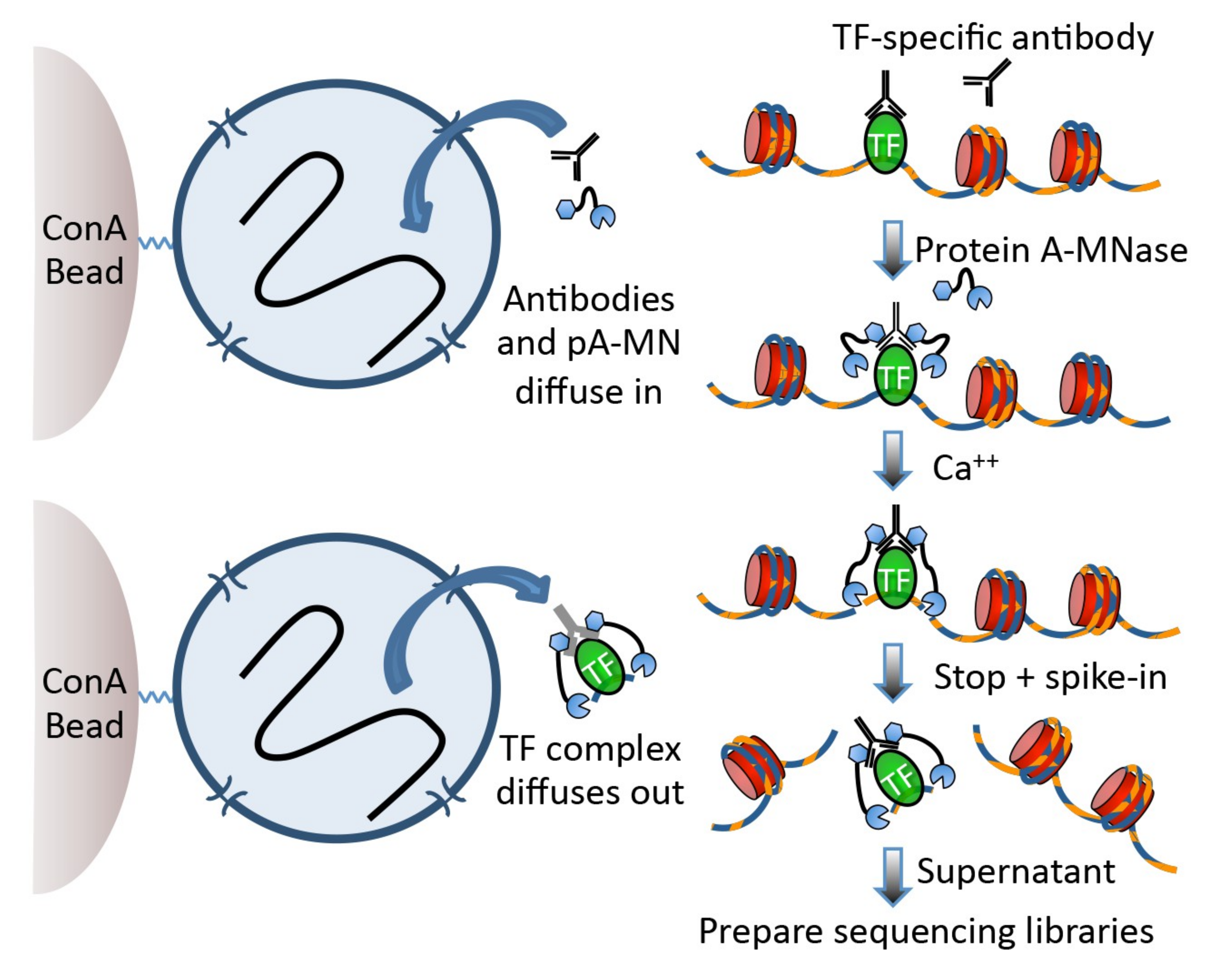
The big difference, CUT&RUN couples the usage of an antibody with the usage of a pA-MNase, which you can see in Figure 1. In the revised version of the protocol Meers et al. 2019,
the pA-MNase has been replaced by a {pA(G)-MNase} to expand this technology to mouse primary antibodies. The enzyme fused to the protein A/G is an
endo-exonuclease that cleaves and shortens DNA. The fusion will ensure that the MNase comes in close proximity with the POI and thus cleaves DNA in-situ, close to POI binding sites. CUT&RUN allows to
fragment the DNA in unfixed cells and thus allows to study protein-DNA interactions in a more natural state. The added pA(G)-MNase thus creates shorted fragments that lead to a higher resolution for the mapping
in comparison to your standard ChIP-Seq protocol. CUT&RUN follows four fundamental steps: (1) permeabilize the nuclei or cells coated on beads, (2) incubate with the selective antibody of the POI, (3)
add the pA(G)-MNase and activate the enzyme for a small period of time, (4) release CUT&RUN fragments and collect the DNA from the supernatant. Afterward, the DNA can be purified, PCR amplified and
prepared for sequencing. You can find the CUT&RUN protocol at protocols.io.
In this tutorial, we will use data from the study of Zhu et al. 2019. The article introduces a CUT&RUN pipeline that we will not completely follow. It is important to note at this point that
a CUT&RUN data analysis is more similar to an ATAC-Seq experiment than a standard ChIP-Seq. We will analyze the two biological replicates from a CUT&RUN experiment for the aforementioned TF GATA1 in humans.
We downsampled the data to speed up the run times in this tutorial. Our results will be compared to identified binding sites of GATA1 of a ChIP-Seq experiment Canver et al. 2017.
When working with real data
The workflow for this training material can be found at the European Galaxy instance. When you use your data we suggest using this workflow
which includes additional steps for your data analysis. Both workflows do not support peak calling with controls as CUT&RUN has a low background.
It is often recommended to use a positive or negative control as a comparison. Spike-in controls can be done for CUT&RUN but need then additional steps in the provided workflows to consider them.
Your results may be slightly different from the ones presented in this tutorial due to differing versions of tools, reference data, external databases, or because of stochastic processes in the algorithms.
Step 1: Preprocessing
Get Data
We first need to download the sequenced reads (FASTQs) as well as other annotation files. Then, to increase the number of reads that will map to the reference genome (here human genome version 38, GRCh38/hg38), we need to preprocess the reads.
Hands On: Data upload
Create a new history for this tutorial
To create a new history simply click the new-history icon at the top of the history panel:
Import the files from Zenodo or from
the shared data library (GTN - Material -> epigenetics
-> CUT&RUN data analysis):
Click galaxy-uploadUpload at the top of the activity panel
Select galaxy-wf-editPaste/Fetch Data
Paste the link(s) into the text field
Press Start
Close the window
As an alternative to uploading the data from a URL or your computer, the files may also have been made available from a shared data library:
Go into Libraries (left panel)
Navigate to the correct folder as indicated by your instructor.
On most Galaxies tutorial data will be provided in a folder named GTN - Material –> Topic Name -> Tutorial Name.
Select the desired files
Click on Add to Historygalaxy-dropdown near the top and select as Datasets from the dropdown menu
In the pop-up window, choose
“Select history”: the history you want to import the data to (or create a new one)
Click on Import
Add a tag called #rep1 to the Rep1 files and a tag called #rep2 to the Rep2 files.
Datasets can be tagged. This simplifies the tracking of datasets across the Galaxy interface. Tags can contain any combination of letters or numbers but cannot contain spaces.
To tag a dataset:
Click on the dataset to expand it
Click on Add Tagsgalaxy-tags
Add tag text. Tags starting with # will be automatically propagated to the outputs of tools using this dataset (see below).
Press Enter
Check that the tag appears below the dataset name
Tags beginning with # are special!
They are called Name tags. The unique feature of these tags is that they propagate: if a dataset is labelled with a name tag, all derivatives (children) of this dataset will automatically inherit this tag (see below). The figure below explains why this is so useful. Consider the following analysis (numbers in parenthesis correspond to dataset numbers in the figure below):
a set of forward and reverse reads (datasets 1 and 2) is mapped against a reference using Bowtie2 generating dataset 3;
dataset 3 is used to calculate read coverage using BedTools Genome Coverageseparately for + and - strands. This generates two datasets (4 and 5 for plus and minus, respectively);
datasets 4 and 5 are used as inputs to Macs2 broadCall datasets generating datasets 6 and 8;
datasets 6 and 8 are intersected with coordinates of genes (dataset 9) using BedTools Intersect generating datasets 10 and 11.
Now consider that this analysis is done without name tags. This is shown on the left side of the figure. It is hard to trace which datasets contain “plus” data versus “minus” data. For example, does dataset 10 contain “plus” data or “minus” data? Probably “minus” but are you sure? In the case of a small history like the one shown here, it is possible to trace this manually but as the size of a history grows it will become very challenging.
The right side of the figure shows exactly the same analysis, but using name tags. When the analysis was conducted datasets 4 and 5 were tagged with #plus and #minus, respectively. When they were used as inputs to Macs2 resulting datasets 6 and 8 automatically inherited them and so on… As a result it is straightforward to trace both branches (plus and minus) of this analysis.
Check that the datatype of the 4 FASTQ files is fastqsanger and the peak file (chip_seq_peaks.bed) is bed. If they are not then change the datatype as described below.
Click on the galaxy-pencilpencil icon for the dataset to edit its attributes
In the central panel, click galaxy-chart-select-dataDatatypes tab on the top
In the galaxy-chart-select-dataAssign Datatype, select datatypes from “New Type” dropdown
Tip: you can start typing the datatype into the field to filter the dropdown menu
Click the Save button
Create a paired collection named 2 PE fastqs, and rename your pairs with the sample name followed by the attributes: Rep1 and Rep2.
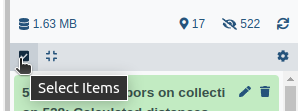
Click on galaxy-selectorSelect Items at the top of the history panel
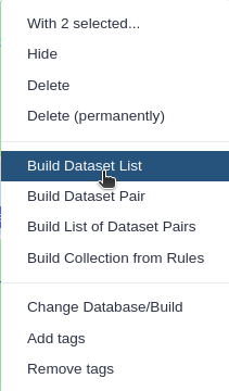
Check all the datasets in your history you would like to include
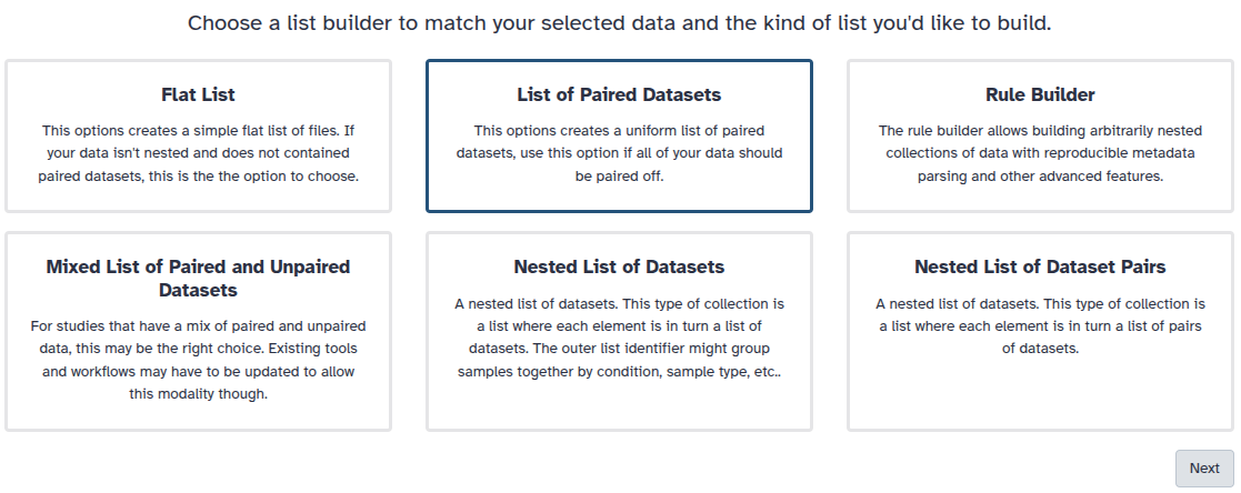
Click n of N selected and choose Advanced Build List
You are in the collection building wizard. Choose List of Paired Datasets and click ‘Next’ button at the right bottom corner.
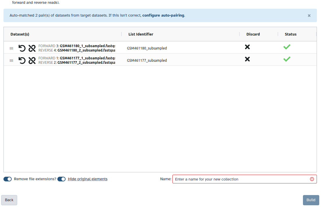
Check and configure auto-pairing. Commonly matepairs have suffix _1 and _2 or _R1 and _R2. Click on ‘Next’ at the bottom.
Edit the List Identifier as required.
Enter a name for your collection
Click Build to build your collection
Click on the checkmark icon at the top of your history again
If you are not familiar with BED format or encode narrowPeak format, see the BED Format
Quality Control
We first have to check if our data contains adapter sequences that we have to remove. A typical CUT&RUN experiment has a read length of 30-80 nt. We can check the raw data quality with Falco.
Hands On: Quality Control
Flatten collection with the following parameters convert the list of pairs into a simple list:
“Input Collection”: 2 PE fastqs
Falco ( Galaxy version 1.2.4+galaxy0) with the following parameters:
param-collection“Raw read data from your current history”: Choose the output of Flatten collectiontool selected as Dataset collection.
Inspect the web page output of Falcotool for the Rep1_forward sample. Check what adapters are found at the end of the reads.
Question
How many reads are in the FASTQ?
Which sections have a warning or an error?
There are 300,000 reads.
The 4 steps below have warnings:
Per base sequence content
CUT&RUN has sometimes base biases like ChIP-Seq.
Sequence Duplication Levels
The read library quite often has PCR duplicates that are introduced
simply by the PCR itself. We will remove these duplicates later on.
Overrepresented sequences
Our data contains TruSeq adapter, Illumina PCR Primer, and a read from the mitochondrial chromosome.
Adapter Content
Our data contains an adapter (Illumina Universal Adapter) that we still have to remove.
As it is tedious to inspect all these reports individually we will combine them with MultiQC ( Galaxy version 1.27+galaxy3).
MultiQC ( Galaxy version 1.27+galaxy3) to aggregate the FastQC reports with the following parameters:
In “Results”:
“Results”
“Which tool was used generate logs?”: FastQC
In “FastQC output”:
param-repeat“Insert FastQC output”
param-collection“FastQC output”: Falco on collection N: Raw data (output of Falcotool)
Comment: Falco Results
This is what you should expect from the Adapter Content section of multiQC:
Figure 2: MultiQC screenshot on the Adapter Content section
The MultiQC report (of FastQC) pointed out that we have in our data some standard Illumina adapter sequences, which we will remove with Trim Galore!.
Trimming Reads
Trim Galore! is a handy tool that can automatically detect and trim standard Illumina adapters.
Hands On: Task description
Trim Galore! ( Galaxy version 0.6.7+galaxy1) with the following parameters:
“Is this library paired- or single-end?”: Paired Collection
“Select a paired collection”: 2 PE fastqs
In “Adapter sequence to be trimmed”: Illumina universal
Avanced settings: Full parameter list
In “Trim low-quality ends from reads in addition to adapter removal (Enter phred quality score threshold)”: 30
In “Discard reads that became shorter than length N”: 15
In “Generate a report file”: Yes
Click on the galaxy-eye (eye) icon of the report for Rep1 and look for the info.
Question
What percentage of reads contain adapters?
What percentage of reads are still longer than 15bp after the trimming?
163,656 (54.6%) for Rep 1 and 169,776 (56.6%) for Rep 2
The last line indicates that 10477 (3.49%) of pairs have been removed from Rep1 and 15775 (5.26%) pairs from Rep2.
Step 2: Mapping
Mapping Reads to Reference Genome
Next, we map the trimmed reads to the human reference genome. Here we will use Bowtie2. We will extend the maximum fragment length (distance between read pairs) from 500 to 1000 because
we know some valid read pairs are from this fragment length. We will use the --very-sensitive parameter to have more chances to get the best match even if it takes a bit longer to run.
We will run the end-to-end mode because we trimmed the adapters, so we expect the whole read to map, no clipping of ends is needed. Regarding the genome to choose.
The hg38 version of the human genome contains alternate loci. This means that some regions of the genome
are present both in the canonical chromosome and on its alternate loci. The reads that map to these regions would map twice. To be able to filter reads falling into
repetitive regions but keep reads falling into regions present in alternate loci, we will map on the Canonical version of hg38 (only the chromosome with numbers, chrX, chrY, and chrM).
Hands On: Mapping reads to reference genome
Bowtie2 ( Galaxy version 2.5.3+galaxy1) with the following parameters:
“Is this single or paired library”: Paired-end Dataset Collection
“FASTQ Paired Dataset: select the output of Trim Galore!tool“paired reads”
“Do you want to set paired-end options?”: Yes
“Set the maximum fragment length for valid paired-end alignments”: 1000
“Will you select a reference genome from your history or use a built-in index?”: Use a built-in genome index
“Select reference genome”: Human (Homo sapiens): hg38 Canonical
“Set read groups information?”: Do not set
“Select analysis mode”: 1: Default setting only
“Do you want to use presets?”: Very sensitive end-to-end (--very-sensitive)
“Do you want to tweak SAM/BAM Options?”: No
“Save the bowtie2 mapping statistics to the history”: Yes
Click on the galaxy-eye (eye) icon of the mapping stats Rep1.
Comment: Bowtie2 Results
You should get similar results to this from Bowtie2:
Both the replicates have almost identical enrichment profile indicating reproducibility. The sharp peak at the end indicates that only a few genomic regions (putative binding sites) were covered with most of the reads which is a very strong enrichment.
There are mainly two reasons to expect such a high enrichment:
Unlike ChIP-seq, CUT&RUN has low background noise.
Our protein of interest (GATA1) in this data set is a transcription factor (TF). TFs usually show high binding specificity.
Filter Uninformative Reads
We apply some filters to the reads after the mapping. CUT&RUN datasets can have many reads that map to the mitochondrial genome because it is nucleosome-free and thus very accessible
to the pA(G)-MNase. CUT&RUN inserts adapter more easily in open chromatin regions due to the pA(G)-MNase activity. The mitochondrial genome is uninteresting for CUT&RUN,
so we remove these reads. We also remove reads with low mapping quality and reads that are not properly paired.
Hands On: Filtering of uninformative reads
Filter BAM datasets on a variety of attributes ( Galaxy version 2.5.2+galaxy2) with the following parameters:
param-collection“BAM dataset(s) to filter”: Select the output of Bowtie2tool“alignments”
In “Condition”:
param-repeat“Condition”
In “Filter”:
“Filter”
“Select BAM property to filter on”: Mapping quality
“Filter on read mapping quality (phred scale)”: >=30
param-repeat“Insert Filter”
“Select BAM property to filter on”: Proper Pair
“Select properly paired reads”: Yes
param-repeat“Insert Filter”
“Select BAM property to filter on”: Reference name of the read
“Filter on the reference name for the read”: !chrM
“Would you like to set rules?”: False
Click on the input and the output BAM files of the filtering step. Check the size of the files.
Question
Based on the file size, what proportion of alignments was removed (approximately)?
Which parameter should be modified if you are interested in repetitive regions?
The original BAM files are 14-15 MB, the filtered ones are 5.8 and 7.1 MB. Approximately half of the alignments were removed.
You should modify the mapQuality criteria and decrease the threshold.
Filter Duplicate Reads
Because of the PCR amplification, there might be read duplicates (different reads mapping to the same genomic region) from over amplification of some regions. We will remove them with Picard MarkDuplicates.
Hands On: Remove duplicates
MarkDuplicates ( Galaxy version 3.1.1.0) with the following parameters:
param-collection“Select SAM/BAM dataset or dataset collection”: Select the output of Filtertool“BAM”
“If true do not write duplicates to the output file instead of writing them with appropriate flags set”: Yes
Comment: Default of **MarkDuplicates** tool
By default, the tool will only “Mark” the duplicates. This means that it will change the Flag of the duplicated reads to enable them to be filtered afterwards. We use the parameter “If true do not write duplicates to the output file instead of writing them with appropriate flags set” to directly remove the duplicates.
Click on the galaxy-eye (eye) icon of the MarkDuplicate metrics.
Comment: MarkDuplicates Results
You should get a similar output to this from MarkDuplicates:
Once again, if you have a high number of duplicates it does not mean that your data are not good, it just means that you sequenced
too much compared to the diversity of the library you generated. Consequently, libraries with a high portion of duplicates should not be re-sequenced as this would not increase the amount of data.
Check Deduplication and Adapter Removal
Hands On: Check Adapter Removal with Falco
Falco ( Galaxy version 1.2.4+galaxy0) with the following parameters:
param-collection“Raw read data from your current history”: select the output of MarkDuplicates BAM.
MultiQC ( Galaxy version 1.27+galaxy3) to aggregate the FastQC reports with the following parameters:
In “Results”:
“Results”
“Which tool was used generate logs?”: FastQC
In “FastQC output”:
param-repeat“Insert FastQC output”
param-collection“FastQC output”: Falco on collection N: Raw data (output of Falcotool)
Comment: FastQC Results
Now, you should see under Overrepresented sequences that there is no more overrepresented sequences and under Adapter Content that the Illumina adapters are no longer present.
Figure 7: MultiQC screenshot on the adapter content section after Trim Galore!
However, you may have noticed that you have a new section with warning: Sequence Length Distribution. This is expected as you trimmed part of the reads.
Furthermore, you will notice under Sequence Duplication Levels that we removed nearly all PCR duplicates.
Figure 8: MultiQC screenshot on the duplication level after MarkDuplicates
Check Insert Sizes
We will check the insert sizes with Paired-end histogram of insert size frequency. The insert size is the distance between the R1 and R2 read pairs. This tells us the size of the DNA fragment the read pairs came from. The fragment length distribution of a sample gives an excellent indication of the quality of the CUT and RUN experiment.
Hands On: Plot the distribution of fragment sizes
Paired-end histogram ( Galaxy version 1.0.2) with the following parameters:
param-collection“BAM file”: Select the output of MarkDuplicatestool“BAM output”
“Lower bp limit (optional)”: 0
“Upper bp limit (optional)”: 1000
Click on the galaxy-eye (eye) icon of the lower one of the 2 outputs (the png file).
Could you guess what the peaks at approximately 30bp correspond to?
The first peak (30bp) corresponds to where the cleavage around our POI. Nevertheless, the cutting of our pA(G)-MNase-antibody-protein complex is not perfect. The arms can actually cut further away from the protein. Little bumps in the distribution are an indication of another protein(complex), such as a nucleosome that is located between the two cleavage sites.
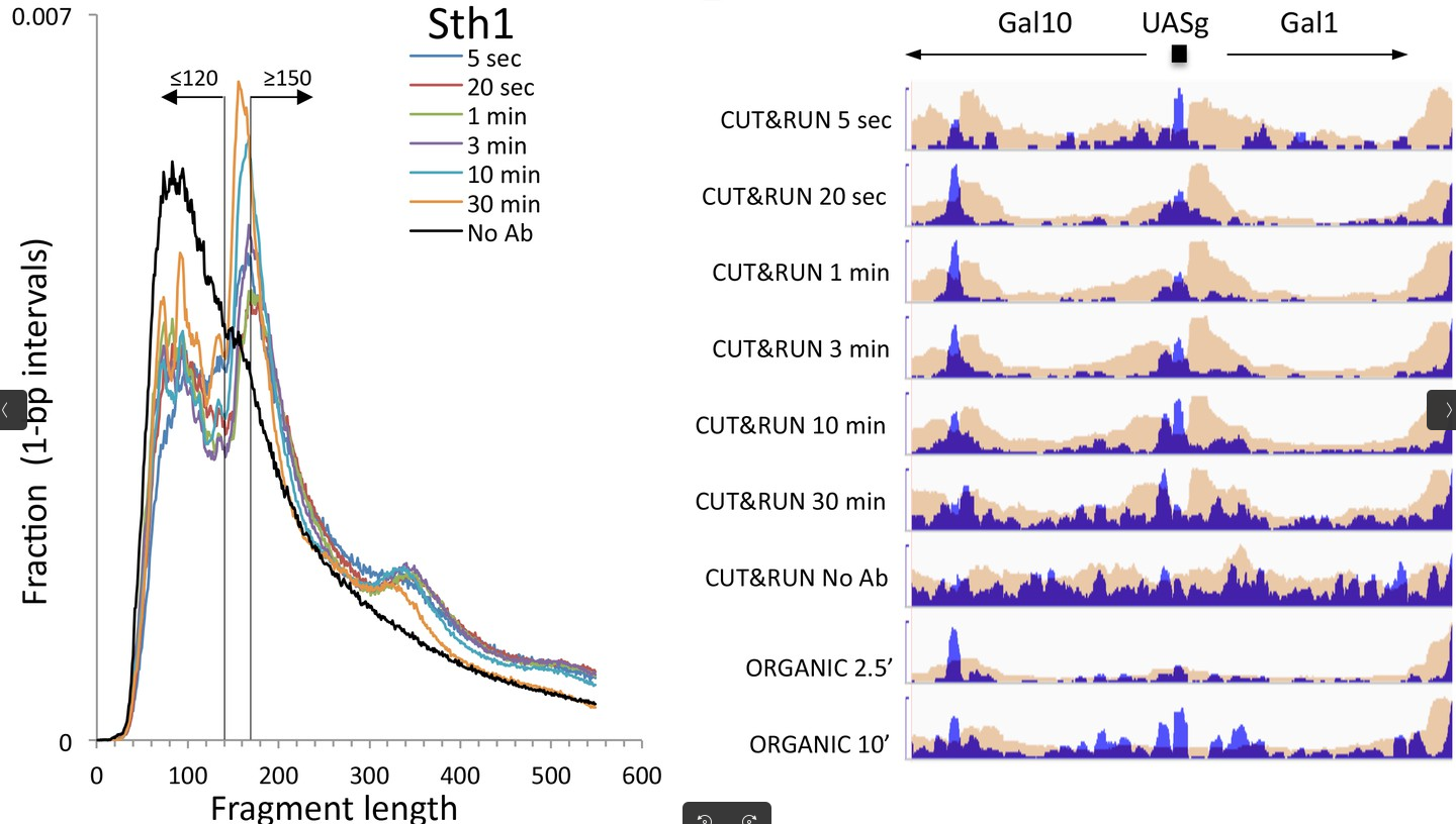
This fragment size distribution is a good indication if your experiment worked or not. The CUT&RUN yield can gradually increase over the digestion time Skene and Henikoff 2017, which of course depends on the enzyme used for the cleavage of the DNA.
Figure 10: Fragment length distributions of a CUT&RUN experiment with uniform digestion over time. No anti-FLAG primary antibody (No Ab). The track with No_Ab is the control experiment. Data is from two biological replicates. The studied protein showed fragments of size ≤120 bp corresponding to the binding sites, as seen on the left, whereas reads with ≥150 bp fragment size are randomly distributed in the local vicinity. The yield in the example increases from 5s to 10 minutes, which can be seen in the mapped profiles in the right. (Skene and Henikoff 2017 eLife)
Step 4: Peak calling
Call Peaks
We have now finished the data preprocessing. Next, to find regions corresponding to potential binding sites, we want to identify regions where reads have piled up (peaks) greater than the background read coverage. MACS2 is widely used for CUT&RUN.
At this step, two approaches exist: Like in ATAC-Seq, we have to take a few things into account. The pA(G)-MNase does not need to bind the protein it can create fragments unspecifically a
few bases downstream and upstream away from the true binding site. This is to the “long” arms of the proteins. A big jump can happen if a nucleosome is between the protein binding site and the cutting site.
It is critical to re-center the signal since the pA(G)-MNase cuts in different distances. Since some read pairs are not symmetric (i.e., the first mate might be further away from the
binding site than the second mate) we will turn off the shifting mode of MACS2 and apply a direct shift. If we only assess the coverage of the 5’ extremity of the reads, the data would be too sparse,
and it would be impossible to call peaks. Thus, we will extend the start sites of the reads by 200bp (100bp in each direction) to assess coverage.
Using MACS2
We convert the BAM file to BED format because when we set the extension size in MACS2, it will only consider one read of the pair while here we would like to use the information from both.
Hands On: Convert the BAM to BED
bedtools BAM to BED converter ( Galaxy version 2.31.1+galaxy0) with the following parameters:
param-collection“Convert the following BAM file to BED”: Select the output of MarkDuplicatestool BAM output
We call peaks with MACS2. To get the coverage centered on the 5’ extended 100bp each side we will use --shift -100 and --extend 200:
MACS2 callpeak ( Galaxy version 2.2.9.1+galaxy0) with the following parameters:
“Are you pooling Treatment Files?”: No
param-collection Select the output of bedtools BAM to BED converter tool
“Do you have a Control File?”: No
“Format of Input Files”: Single-end BED
“Effective genome size”: H. sapiens (2.7e9)
“Build Model”: Do not build the shifting model (--nomodel)
“Set extension size”: 200
“Set shift size”: -100. It needs to be - half the extension size to be centered on the 5’.
“Additional Outputs”:
Check Peaks as tabular file (compatible with MultiQC)
Check Peak summits
Check Scores in bedGraph files
In “Advanced Options”:
“Composite broad regions”: No broad regions
“Use a more sophisticated signal processing approach to find subpeak summits in each enriched peak region”: Yes
“How many duplicate tags at the exact same location are allowed?”: all
Comment: Why keeping all duplicates is important
We previously removed duplicates using MarkDuplicatestool using paired-end information. If two pairs had identical R1 but different R2, we knew it was not a PCR duplicate. Because we converted the BAM to BED we lost the pair information. If we keep the default (removing duplicates) one of the 2 identical R1 would be filtered out as duplicate.
Question
How many peaks have been identified in each replicate?
6314 for Rep1 and 7678 for Rep2
Step 5: Identifying Binding Motifs
Prepare the Datasets
Extracting individual replicates from your dataset collection
In the following step, we want to apply a tool to identify robust peaks between our two replicates. However, we still have one dataset collection, holding both replicates, which we have to split.
Hands On: Extract replicates from a dataset collection:
Extract Dataset with:
param-collection“Input List”: MACS2 callpeak on collection N (narrow Peaks)
“How should a dataset be selected?”: Select by index
“Element index:”: 0
You can use the arrow to rerun the same tool just changing the last parameter:
Extract Dataset with:
param-collection“Input List”: MACS2 callpeak on collection N (narrow Peaks)
“How should a dataset be selected?”: Select by index
“Element index:”: 1
Extract Robust Peaks
MACS helped us to identify potential binding sites for GATA1. Yet, our peak set will contain false positives because of technical and biological noise.
We can first try to reduce some noise using the results for our two biological replicates. Since we applied MACS we have created two peak files.
Yet, both replicates have peaks that are only present in one replicate and thus might be a potential false positive due to noise.
We can remove such peaks if we simply overlap the two peak files and consequently search for peaks that appear in both replicates.
Hands On: Select robust GATA1 peaks:
bedtools Intersect intervals find overlapping intervals in various ways ( Galaxy version 2.31.1+galaxy0) with the following parameters:
param-file“File A to intersect with B”: Select Rep1
“Combined or separate output files”: One output file per 'input B' file
param-file“File B to intersect with A”: Select Rep2
“Calculation based on strandedness?”: Overlaps occurring on either strand
“Required overlap”: Specify minimum overlap(s)
“Minimum overlap required as a fraction of A”: 0.5
“Require that the fraction of overlap be reciprocal for A and B”: Yes
*“Write the original A entry once if any overlaps found in B.”: Yes
Rename the datasets Robust GATA1 CUT and RUN peaks.
Question
How many potential true positives do we obtain?
How many potential false positives have we removed?
Why have we set specified an overlap fraction of A with 0.5?
Why have we set “Require that the fraction of overlap be reciprocal for A and B”?
2,865 peaks
We started with 6,314 and 7,678 peaks. Thus, we could remove 3,449 and 4,813 peaks.
Finding robust peaks is a tricky process and not as simple as you think. Our approach defines a robust peak as an entity that is covered by two similar peaks in either one of the peak files of our two replicates. Our measurement for similarity is simply the amount of bases the peaks overlap. Yet, ask yourself, how much overlap do you need to state that they are similar? Is 1 base enough or maybe 10? The answer is not true or false and like so often needs more investigation. We define the overlap by a 50% fraction of each of the peak files. That means, if our peak in A is 100 bases then A has to overlap with 50 bases with the peak in file B.
“Require that the fraction of overlap be reciprocal for A and B” means that 50% of the peak in file A overlaps with the peak in file B and also 50% of the peak in file B overlaps with the peak in file A. We set this to make our filtering very conservative and filter for peaks that we can be sure are true positives. For example, A has a 10 bp peak that overlaps a peak in B with 100 bp. Viewpoint of file A: An overlap-fraction of 0.5 for A means that we accept peak A if it overlaps with 5 bp with the peak in B. This is very likely because the peak in B is 100 bp long. Viewpoint of file B: An overlap-fraction of 0.5 for B means that we reject A no matter what, even if A completely overlaps B because 10 bp are not enough to cover 50% of B. That is to say the option “Require that the fraction of overlap be reciprocal for A and B” takes care that we trust peaks that have in file A and in file B a fair overlap.
Note, that this is one way to define robust peaks. Yet, there are more sophisticated algorithms in Galaxy, such as
IDR compare ranked list of identifications ( Galaxy version 2.0.3), and other methods that can help to define a robust peak.
The tool IDR has not been tested so far for CUT and RUN.
Extract Positive Peaks
We can further remove some noise with a positive control, that is why we have downloaded a peak set from a ChIP experiment of GATA1.
Hands On: Select GATA1 peaks from ChIP-Seq data:
bedtools Intersect intervals find overlapping intervals in various ways ( Galaxy version 2.31.1+galaxy0) with the following parameters:
param-file“File A to intersect with B”: Select Robust GATA1 CUT and RUN peaks
“Combined or separate output files”: One output file per 'input B' file
param-file“File B to intersect with A”: Select the dataset GATA1 ChIP-Seq peaks
“Calculation based on strandedness?”: Overlaps occurring on either strand
“Required overlap”: Specify minimum overlap(s)
“Minimum overlap required as a fraction of A”: 0.5
“Require that the fraction of overlap be reciprocal for A and B”: No
*“Write the original A entry once if any overlaps found in B.”: Yes
Rename the datasets True GATA1 CUT and RUN peaks.
Question
How many potential true positives have we found (common between CUT&RUN and ChIP-seq) ?
How many potential false positives have we removed?
What is the precision of our analysis at this point? (Precision = True Positive / True Positive + False Positive)
2,809 peaks
56 peaks
Our precision is ~ 98%. A high precision is an indicator that we can predict true binding regions with high confidence.
Extract DNA sequence
Hands On: Obtain DNA sequences from a BED file
Extract Genomic DNA using coordinates from assembled/unassembled genomes ( Galaxy version 3.0.3+galaxy3) with the following parameters:
param-file“Fetch sequences for intervals in”: True GATA1 CUT and RUN peaks
“Interpret features when possible”: No
*“Choose the source for the reference genome”: locally cached
“Using reference genome”: hg38
“Select output format”: fasta
“Select fasta header format”: bedtools getfasta default
Motif detection with MEME-ChIP
Let’s find out the sequence motifs of the TF GATA1. Studies have revealed that GATA1 has the DNA binding motif (T/A)GATA(A/G) Hasegawa and Shimizu 2017. In this last task we search for this motif in our data.
Hands On: Motif detection
MEME-ChIP ( Galaxy version 4.11.2+galaxy1) with the following parameters:
param-file“Primary sequences”: Select the output of Extract Genomic DNAtool
“Sequence alphabet”: DNA
“Options Configuration”: Advanced
“Should subsampling be random?”: Yes
“Seed for the randomized selection of sequences”: 123
“E-value threshold for including motifs”: 0.05
“What is the expected motif site distribution?”: Zero or one occurrence per sequence
“Minimum motif width”: 5
“Maximum motif width”: 20
“Maximum number of motifs to find”: 5
“Stop DREME searching after reaching this E-value threshold”: 0.05
“Stop DREME searching after finding this many motifs”: 5
- “I certify that I am not using this tool for commercial purposes.”: Yes
View the MEME-ChIP HTML.
Question
What is the E-value of the main motif?
How many peaks support the main motif GATA?
1.1e-411
You need to click on the DREME link for the GATA motif. Then when you are in the DREME html, click on the arrow pointing down for the first motif (HGATAA) in the More column. Here, it gives you some numbers including how many peaks were positive for the motif. Here 1939.
Figure 12: Plot of the first five sequence motifs of MEME-ChIP.
Let us first investigate the result of MEME-ChIP. First column: The x-axis of the sequence plots represents the nucleotide position of the motif.
The y-axis stands for the total information (uncertainty) and thus stands for the probability that the nucleotide at a certain position is the specific letter (for DNA: T,C,G,A).
Bigger letters stand for a higher probability. For more information please read the corresponding Wikipedia page. Second column: Defines the algorithm that found the sequence motif.
MEME-ChIP uses two different approaches called MEME and DREME, which can find more complex or simpler motifs. More information about these tools can be found in the Meme documentation.
Third column: Defines the E-value, which represents the expected number of times we would find our sequence motif in a database (peak file), just by chance.
This means, that a small E-value corresponds to a very significant motif because the expected number we would find that motif in our peak file just by chance is very low.
Other sequences like repeats will have a high E-value on the other hand. Fourth column: This graph is the result of CentriMo, a tool that shows the distribution of
the best matches for that particular motif. The vertical line is the center of the motif. Therefore, if you have a long sequence motif CentriMo helps you to pinpoint a smaller sub-motif.
You can find more information on CentriMo in the Meme documentation.
The results of MEME-ChIP endorse the findings about the DNA binding motif (T/A)GATA(A/G) Hasegawa and Shimizu 2017. We also found other motifs, that might be secondary sequence motifs.
This, we could test with a deeper analysis.
Step 6: Visualisation of Coverage
In the previous section we generated the True GATA1 CUT and RUN peaks file by eliminating the false positives. In this step, we will visualize the the coverage across the peaks using the bedgraph file generated by MACS2tool.
Convert bedgraph from MACS2 to bigwig
The BedGraph format is human-readable but can be quite large, making it slow to visualize specific regions. For better efficiency, we will convert it to the BigWig format, a binary format that allows for fast visualization of any genomic region.
Hands On: Convert BedGraphs to BigWig.
Wig/BedGraph-to-bigWig with the following parameters:
param-file“Convert”: Select the output of MACS2tool (Bedgraph Treatment).
“Converter settings to use”: Default
Rename the datasets MACS2 bigwig.
Create heatmap of coverage at TSS with deepTools
You might be interested in checking the coverage on binding GATA1 binding sites. For this, you can compute a heatmap. We will use the deepTools plotHeatmap. Here we make a heatmap centered on the transcription start sites (TSS).
Generate computeMatrix
The input of plotHeatmap is a matrix in a hdf5 format. To generate it we use the tool computeMatrix that will evaluate the coverage at each GATA1 peak.
Hands On: Generate the matrix
computeMatrix ( Galaxy version 3.5.4+galaxy0) with the following parameters:
In “Select regions”:
param-repeat“Insert Select regions”
param-file“Regions to plot”: True GATA1 CUT and RUN peaks
“Sample order matters”: No
param-file“Score file”: MACS2 bigwig, output of Wig/BedGraph-to-bigWigtool.
“computeMatrix has two main output options”: reference-point
“The reference point for the plotting”: beginning of region (e.g. TSS)
“Show advanced output settings”: no
“Show advanced options”: yes
“Convert missing values to 0?”: Yes
Plot with plotHeatmap
Now we will generate a heatmap. Each line will be a peak. The coverage will be summarized with a color code from red (no coverage) to blue (maximum coverage). All TSS will be aligned in the middle of the figure and only the 1 kb around the TSS will be displayed. Another plot, on top of the heatmap, will show the mean signal at the TSS. There will be one heatmap per replicate.
Hands On: Generate the heatmap
plotHeatmap ( Galaxy version 3.3.2.0.1) with the following parameters:
param-file“Matrix file from the computeMatrix tool”: output of computeMatrixtool.
“Show advanced output settings”: no
“Show advanced options”: Yes
“The x-axis label”: distance from peak center (bp)
“The y-axis label for the top panel” : GATA1 peaks
“Reference point label”: peak center
“Labels for the regions plotted in the heatmap”: GATA1_peaks
What does the coverage tell us about the binding sites?
Except a slightly more average coverae in replicate 2, both of them have similar sharp pattern.
Such sharp coverage indicates that the binding sites are highly specific, which is expected for transcription factor binding.
Conclusion
In this training, you have learned the general principles of CUT&RUN data analysis. CUT&RUN is a method to analyse DNA-associated proteins. In contrast to ChIP-seq, CUT&RUN couples the
antibody with a pA(G)-MNase to reduce the size of the obtained sequences to increase the accuracy for the detection of the protein interaction. Based on this training material,
you gained some insights into the quality control of the data. You should know some pitfalls of CUT&RUN and look for adapter contamination and PCR duplicates, which disrupt the later enrichment analysis.
You learned about Bowtie2 to do the alignment, and how to filter for properly paired, good-quality and reads that do not map to the mitochondrial genome. Furthermore, you learned that
an indicator for a good CUT&RUN experiment is the fragment size plot and that you optimize your protocol based on this parameter. With MACS2 we identified enriched regions, but
we had to remove some noise. We performed some robust peak analysis with bedtools intersect and performed a check with a ChIP-Seq experiment to remove some false positives.
Finally, we used MEME-ChIP to identify our binding motifs.
You've Finished the Tutorial
Please also consider filling out the Feedback Form as well!
Key points
CUT&RUN can be used to identify binding regions for DNA binding proteins.
Several filters are applied to the reads, such as removing those mapped to mitochondria
Fragment distribution can help determine whether an CUT&RUN experiment has worked well
A robust peak detection removes noise from the data
Frequently Asked Questions
Have questions about this tutorial? Have a look at the available FAQ pages and support channels
Canver, M. C., S. Lessard, L. Pinello, Y. Wu, Y. Ilboudo et al., 2017 Variant-aware saturating mutagenesis using multiple Cas9 nucleases identifies regulatory elements at trait-associated loci. Nature Genetics 49: 625–634. 10.1038/ng.3793
Skene, P. J., and S. Henikoff, 2017 An efficient targeted nuclease strategy for high-resolution mapping of DNA binding sites (D. Reinberg, Ed.). eLife 6: e21856. 10.7554/eLife.21856
Meers, M. P., T. D. Bryson, J. G. Henikoff, and S. Henikoff, 2019 Improved CUT&RUN chromatin profiling tools (S. Parker & D. Weigel, Eds.). eLife 8: e46314. 10.7554/eLife.46314
Zhu, Q., N. Liu, S. H. Orkin, and G.-C. Yuan, 2019 CUT&RUNTools: a flexible pipeline for CUT&RUN processing and footprint analysis. Genome Biology 20: 192. 10.1186/s13059-019-1802-4
Glossary
CUT&RUN
Cleavage Under Targets and Release Using Nuclease
POI
protein of interest
TF
transcription factors
pA(G)-MNase
protein A(-protein G hybrid)-micrococcal nuclease
Feedback
Did you use this material as an instructor? Feel free to give us feedback on how it went.
Did you use this material as a learner or student? Click the form below to leave feedback.
Hiltemann, Saskia, Rasche, Helena et al., 2023 Galaxy Training: A Powerful Framework for Teaching! PLOS Computational Biology 10.1371/journal.pcbi.1010752
Batut et al., 2018 Community-Driven Data Analysis Training for Biology Cell Systems 10.1016/j.cels.2018.05.012
@misc{epigenetics-cut_and_run,
author = "Florian Heyl and Pavankumar Videm",
	title = "CUT&RUN data analysis (Galaxy Training Materials)",
	year = "",
	month = "",
	day = "",
	url = "\url{https://training.galaxyproject.org/training-material/topics/epigenetics/tutorials/cut_and_run/tutorial.html}",
	note = "[Online; accessed TODAY]"
}
@article{Hiltemann_2023,
	doi = {10.1371/journal.pcbi.1010752},
	url = {https://doi.org/10.1371%2Fjournal.pcbi.1010752},
	year = 2023,
	month = {jan},
	publisher = {Public Library of Science ({PLoS})},
	volume = {19},
	number = {1},
	pages = {e1010752},
	author = {Saskia Hiltemann and Helena Rasche and Simon Gladman and Hans-Rudolf Hotz and Delphine Larivi{\`{e}}re and Daniel Blankenberg and Pratik D. Jagtap and Thomas Wollmann and Anthony Bretaudeau and Nadia Gou{\'{e}} and Timothy J. Griffin and Coline Royaux and Yvan Le Bras and Subina Mehta and Anna Syme and Frederik Coppens and Bert Droesbeke and Nicola Soranzo and Wendi Bacon and Fotis Psomopoulos and Crist{\'{o}}bal Gallardo-Alba and John Davis and Melanie Christine Föll and Matthias Fahrner and Maria A. Doyle and Beatriz Serrano-Solano and Anne Claire Fouilloux and Peter van Heusden and Wolfgang Maier and Dave Clements and Florian Heyl and Björn Grüning and B{\'{e}}r{\'{e}}nice Batut and},
	editor = {Francis Ouellette},
	title = {Galaxy Training: A powerful framework for teaching!},
	journal = {PLoS Comput Biol}
}
Congratulations on successfully completing this tutorial!
You can use Ephemeris's shed-tools install command to install the tools used in this tutorial.
4 stars:
Liked: It was straight forward and easy to understand for the beginner like me.
Disliked: It could be more helpful if you also talk about spike-in normalization as it is important for CUT&RUN.
April 2025
5 stars:
Liked: Clear description of each step
Disliked: Detailed desription of each changed parameter when running tools - why is it like that etc.
January 2025
5 stars:
Disliked: Could you include the methods for spike-in normalization?
November 2024
3 stars:
Liked: modification in MACS2 to detect peaks
Disliked: plotting heatmaps and explaining each part , more explanation in video format ,
October 2024
4 stars:
Liked: customization for Cut and run using MACS2 and all the QC
Disliked: I would like ot understand more about each type of graphs how to understand for different Cut and run expt eg how input will differ from TF or the Histone mark antibodies, also would like a video of this sometimes there is better explanation than written.
Questions:
 Open image in new tab


Open image in new tab
Open image in new tab
Open image in new tab
Open image in new tab
Open image in new tab
Open image in new tab
Open image in new tab
Open image in new tab
 Open image in new tab
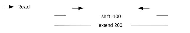 Open image in new tab
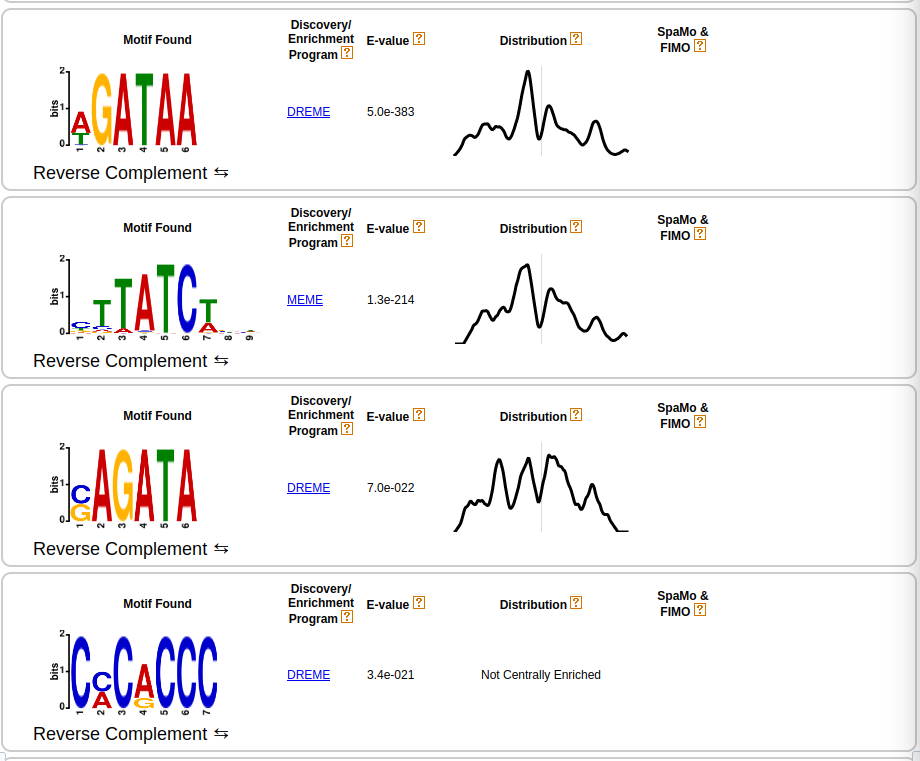 Open image in new tab
Open image in new tab