OpenRefine Tutorial for researching cultural data
| Author(s) |
|
| Tester(s) |
|
| Reviewers |
|
OverviewQuestions:
Objectives:
How to use OpenRefine in Galaxy to clean your data?
How to use a workflow in Galaxy to extract and visualise information from your data?
Requirements:
Start OpenRefine as an Interactive Tool in Galaxy
Use OpenRefine to clean your data (remove duplicates, separate multiple values from the same field, etc.)
Export your cleaned data from OpenRefine to Galaxy
Use a pre-existing workflow in Galaxy to extract specific information and visualise your findings
Time estimation: 2 hoursLevel: Introductory IntroductorySupporting Materials:
- Datasets
- Workflows
- galaxy-history-answer Answer Histories
- FAQs
- instances Available on these Galaxies
Published: Sep 24, 2025Last modification: Apr 29, 2026License: Tutorial Content is licensed under Creative Commons Attribution 4.0 International License. The GTN Framework is licensed under MITpurl PURL: https://gxy.io/GTN:T00560rating Rating: 5.0 (1 recent ratings, 1 all time)version Revision: 3
This tutorial shows how to use OpenRefine in Galaxy to clean and visualize data from the humanities and social sciences. It has two parts:
- Introduction to OpenRefine, based on Hooland et al. 2013 and adapted for Galaxy.
- Introduction to running Galaxy workflows to visualize cleaned data and extract specific information.
What is OpenRefine?
OpenRefine is a free, open-source “data wrangler” built for messy, heterogeneous, evolving datasets. It imports common formats (CSV/TSV, Excel, JSON, XML) and domain-specific ones used across GLAM (Galleries, Libraries, Archives and Museums) and official statistics (MARC, RDF serializations, PC-Axis).
It is non-destructive—OpenRefine does not alter your source files, but works on copies and saves projects locally. Facets and filters enable you to audit categories, surface outliers, and triage inconsistencies without writing code. Its clustering tools consolidate near-duplicates using both key-collision methods (fingerprint, n-gram, phonetic) and edit-distance/nearest-neighbour methods (Levenshtein, PPM) so you can standardize names and places at scale while keeping human oversight.
For enrichment, OpenRefine speaks the Reconciliation API to match local values to external authorities (e.g. Wikidata, ROR) and, optionally, retrieve richer metadata. Transformations—both point-and-click and GREL formulas—are recorded as a stepwise, undoable history that you can export as JSON and re-apply to other datasets, enabling reproducible cleaning and easy peer review. Finished tables can be exported cleanly to CSV/TSV, ODS/XLS(X), SQL statements, templated JSON, Google Sheets, or can be exported back to Galaxy.
From Cleaning to Analysis in Galaxy
Once your dataset has been cleaned with OpenRefine, you often want to analyze it further or visualize specific aspects. This is where Galaxy Workflows become essential: they enable you to build reproducible pipelines that operate on your curated data, transitioning from one-off cleaning to structured analysis.
What are Galaxy Workflows?
Galaxy Workflows are structured, step-by-step pipelines that you build and run entirely in the browser—either extracted from a recorded analysis history or assembled in the visual editor. They can be annotated, shared, published, imported, and rerun, making them ideal for teaching, collaboration, and reproducible research.
A captured analysis is easy to share: export the workflow as JSON (.ga: tools, parameters, and Input/Output) or export a provenance-rich run as a Workflow Run RO-Crate bundling the definition with inputs, outputs, and invocation metadata. This lowers the barrier to entry (no local installs; web User-Interface (UI) with pre-installed tools and substantial compute) while preserving best practices (histories track tool versions and parameters; workflows are easily re-applied to new data).
For findability and credit, the community uses WorkflowHub—a curated registry that supports multiple workflow technologies (including Galaxy) and promotes FAIR principles; it offers Spaces/Teams, permissions, versioning, and DOIs via DataCite, with metadata linking to identifiers like ORCID so contributions enter scholarly knowledge graphs and are properly acknowledged.
In practice, you can iterate on a workflow in a familiar Graphic-User-Interface (GUI), export the exact definition or a run package, and deposit it where peers can discover, reuse, review, and cite it—closing the loop between simple authoring and robust scholarly dissemination.
AgendaIn this tutorial, we will cover:
Hands on: Get the data
We will work with a slightly adapted dataset from the Powerhouse Museum (Australia’s largest museum group) containing a metadata collection. The museum shared the dataset online before giving API access to its collection. We slightly adapted the dataset and uploaded it to Zenodo for long-term reuse. The tabular file (36.4 MB) includes 14 columns for 75,811 objects, released under a Creative Commons Attribution Share Alike (CCASA) license. We will answer three questions: From which category does the museum have the most objects? From which year does the museum have the most objects? And what objects does the museum have from that year?
Why this dataset? It is credible, openly published, and realistically messy—ideal for practising problems scholars encounter at scale. Records include a Categories field populated from the Powerhouse Museum Object Names Thesaurus (PONT), a controlled vocabulary reflecting Australian usage. The tutorial deliberately surfaces common quality issues—blank values that are actually stray whitespace, duplicate rows, and multi-valued cells separated by the pipe character | (including edge cases where double pipes || inflate row counts)—so we can practice systematic inspection before any analysis. Without careful atomization and clustering, these irregularities would bias statistics, visualizations, and downstream reconciliation.
We suggest that you download the data from the Zenodo record as explained below. This helps us with the reproducibility of the results.
Hands On: Upload your data
- Create a new history for this tutorial and name it “Powerhouse Museum — OpenRefine”
Import the files from Zenodo:
https://zenodo.org/records/17047254/files/phm_collection_adapted.tsv
https://zenodo.org/records/17047254/files/stopwords-en.txt
- Copy the link location
Click galaxy-upload Upload at the top of the activity panel
- Select galaxy-wf-edit Paste/Fetch Data
Paste the link(s) into the text field
Press Start
- Close the window
As an alternative to uploading the data from a URL or your computer, the files may also have been made available from a shared data library:
- Go into Libraries (left panel)
- Navigate to the correct folder as indicated by your instructor.
- On most Galaxies tutorial data will be provided in a folder named GTN - Material –> Topic Name -> Tutorial Name.
- Select the desired files
- Click on Add to History galaxy-dropdown near the top and select as Datasets from the dropdown menu
In the pop-up window, choose
- “Select history”: the history you want to import the data to (or create a new one)
- Click on Import
- Ensure that the datatype of “phm_collection_adapted” is “tsv”. Otherwise, use convert datatype.
Verify that the datatype of “stopwords-en” is “txt”. If not, convert the datatype.
- Click on the galaxy-pencil pencil icon for the dataset to edit its attributes
- In the central panel, click galaxy-chart-select-data Datatypes tab on the top
- In the galaxy-chart-select-data Assign Datatype, select
datatypesfrom “New Type” dropdown
- Tip: you can start typing the datatype into the field to filter the dropdown menu
- Click the Save button

In this first part, we will focus on working with the metadata from the Powerhouse Museum.
Use OpenRefine to explore and clean your dataset
Access OpenRefine as an interactive tool in Galaxy and explore your data.
Start OpenRefine
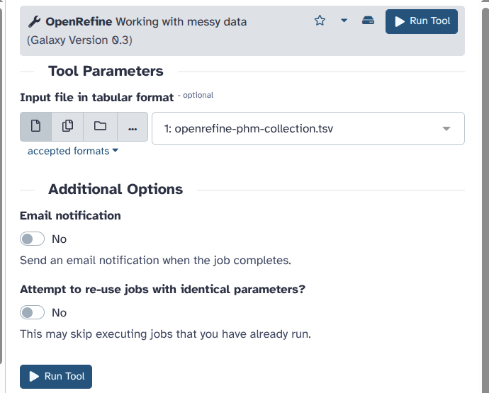
Hands On: Opening the dataset with OpenRefine
- Open the tool OpenRefine: Working with messy data
- “Input file in tabular format”:
openrefine-phm-collection.tsvClick on “Run Tool”.
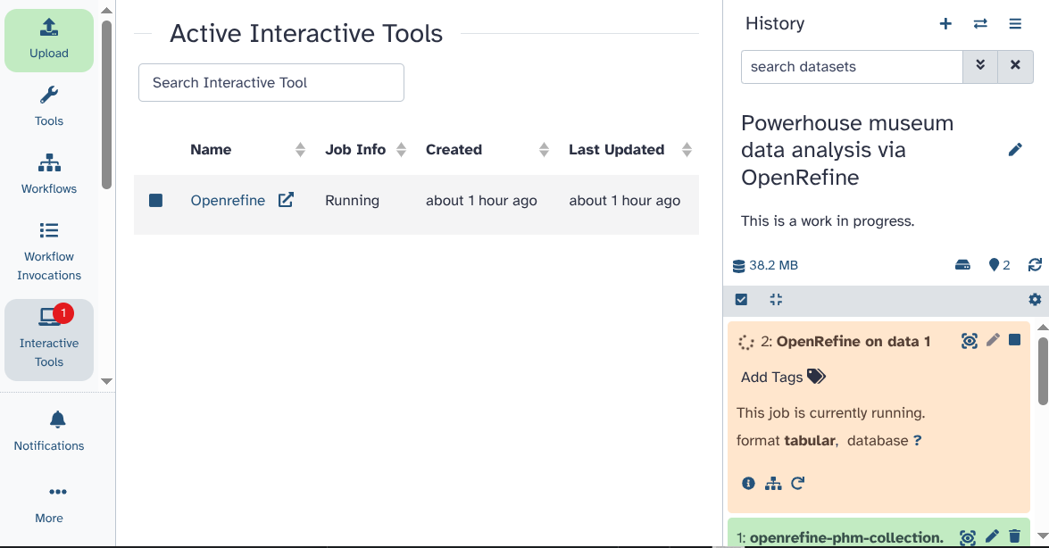
After around 30 seconds, a red dot appears over the interactive tools section on the left panel. Click on “interactive tools”. A new window opens. Make sure to wait until you see the symbol with an arrow pointing outside the box, which indicates that you can start OpenRefine in a new tab. Now you can open OpenRefine by clicking on its name.
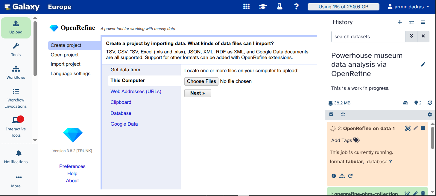
Here, you can see the OpenRefine GUI. Click on
Open Project.
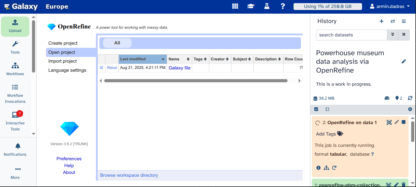
Click on
Galaxy file. If the file does not appear, you may have started OpenRefine before it was fully loaded. Retry steps 3 and 4, and the file should be visible.
You can see the data that has been loaded for you.
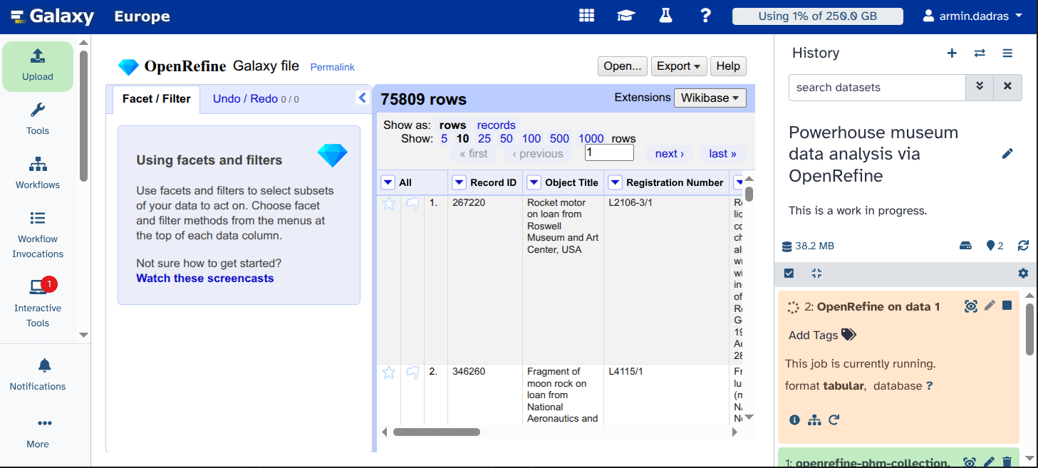
Question
- How many rows does this table have?
- 75809
Great, now that the dataset is in OpenRefine, we can start cleaning it.
Remove duplicates
In large datasets, errors are common. Some basic cleaning exercises can help enhance the data quality. One of those steps is to remove duplicate entries.
Hands On: Removing duplicates
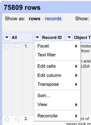
Click on the triangle on the left of
Record ID.
Click on
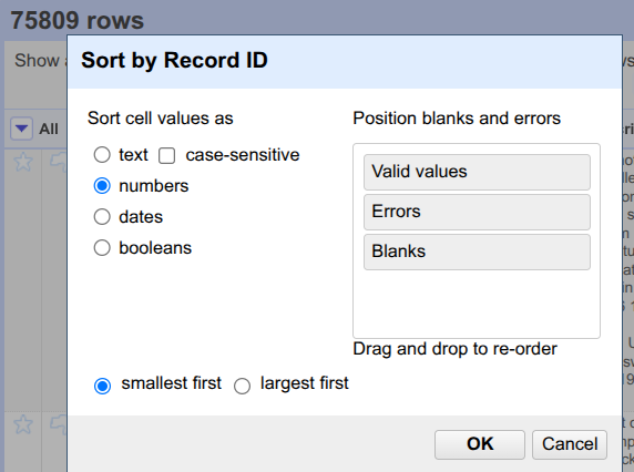
Sort....Select
numbersand click onOK.
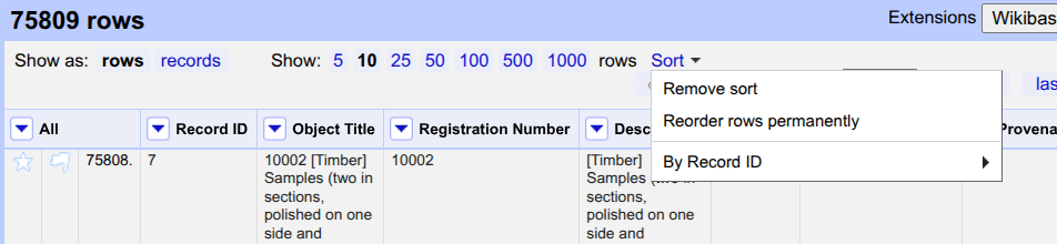
Above the table, click on
Sortand selectReorder rows permanently.
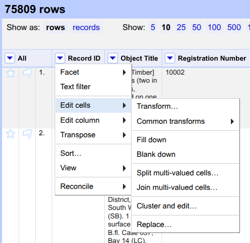
Click on the triangle left of the
Record IDcolumn. Hover overEdit cellsand selectBlank down.
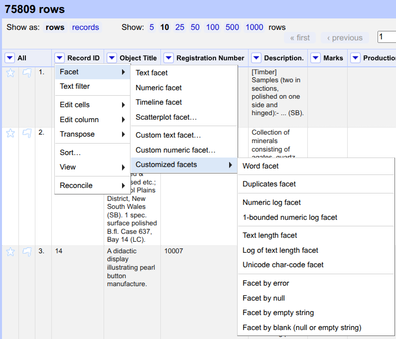
Click on the triangle left of the
Record IDcolumn. Hover overFacet, then move your mouse toCustomized facetsand selectFacet by blank (null or empty string).
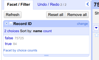
On the left, a new option appears under
Facet/Filterwith the titleRecord ID. It shows two choices,trueandfalse. Click ontrue.
Click on the triangle to the left of the column called
All. Hover overEdit rows, and selectremove matching rows.
Close the
Record IDunderFacet/Filterby clicking on the cross (x) to see all rows.
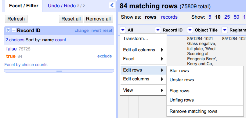
Question
- How many rows have been removed?
- 84
The dataset no longer contains duplicates based on the Record ID. However, we need to perform further cleaning to enhance the dataset.
Use GREL
There are many ways to manipulate your dataset in OpenRefine. One of them is the Google Refine Expression Language (GREL). With the help of GREL, you can, for example, create custom facets or add columns by fetching URLs. We will use it to find and replace errors. For more information, refer to the GREL documentation.
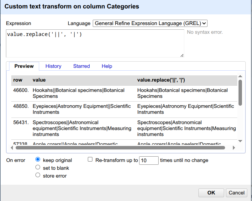
Take a look at the Categories column of your dataset. Most objects were attributed to various categories, separated by “|”. However, several fields contain “||” instead of “|” as a separator. We want to unify those.
Hands On: Find and replace typos using GRELTo remove the occurance of double pipe “||” from the file we can do the following:
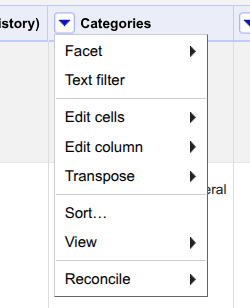
- Click on the triangle on the left of
Categoriesand selectText filter.- On the left, using the
Facet/Filtersection, search for the occurrence of | and ||. There are 71061 rows with “|” and 9 rows with “||”. We would like to remove these nine lines, as they were added by mistake.- Click on the triangle on the left of
Categories, hover overEdit cells, and click onTransform....In the new window, use the following text
value.replace('||', '|')as “Expression” and click onOK.
The expression replaces || with |. If you search for the occurrence of || again, you will no longer get any results.
Many different categories describe the object. You may notice duplicates categorising the same object twice. We also want to remove those to ensure we only have unique categories that describe a single object.
Click on the triangle on the left of
Categories, hover overEdit cells, and click onTransform....
- In the new window, use the following text
value.split('|').uniques().join('|')as “Expression” and click onOK.
These expressions split categories at the pipe separator and join the unique ones within this column. As a result, duplicate categories for one object are deleted.
Question
- How many cells had duplicated categories?
- 1,668
Atomization
Once the duplicate records have been removed, we can examine the content of the “Categories” column more closely. Different categories are separated from each other by pipe (|). Each entry can be assigned to more than one category. To leverage those keywords, the values in the Categories column must be split into individual cells using the pipe character.
Hands On: Atomization
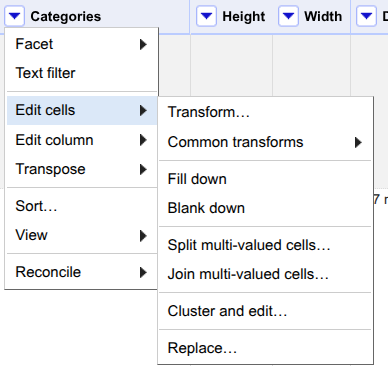
Click on the triangle on the left of
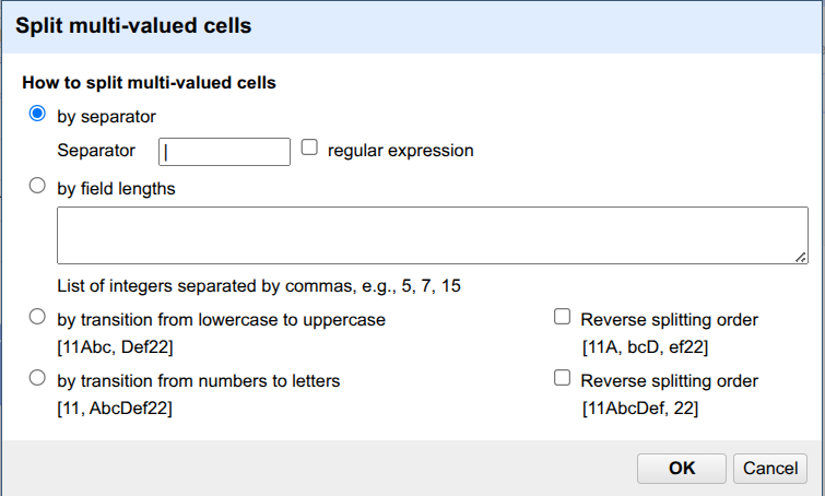
Categories, hover overEdit cells, and click onSplit multi-valued cells....
Define the
Separatoras\|(pipe). Click onOK.
Are you ready for a little challenge? Let’s investigate the categories column of the museum items.
Question
- How many rows do you have after atomizing the categories column?
- How many entries do not have any category?
- 168,476
- Click on the triangle on the left of
Categoriesand hover overfacetand move your mouse overCustomized facets, and click onFacet by blank (null or empty string). Thetruevalue for blank entries is 447.
Faceting
Now that the Categories field is cleaned, we can check the occurrence of categories with various facets.
Hands On: Faceting
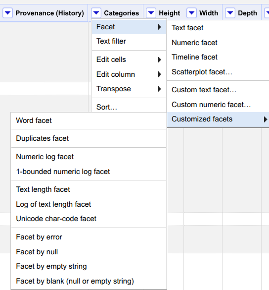
- Click on the triangle on the left of
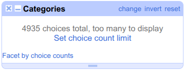
Categories, hover overFacet, and click onText facet.On the left panel, it mentions the total number of choices. The default value of
count limitis low for this dataset, and we should increase it. Click onSet choice count limit.
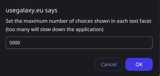
Enter
5000as the new limit and click onOk.
Now, you see all categories. Click on
countto see the categories sorted in descending order.
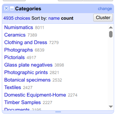
You can now see, from which category the museum has the most objects, one of our initial questions about the dataset.
Question
- What are the top 3 categories? How many items are associated with each of them?
- Numismatics (8011), Ceramics (7389), and Clothing and Dress (7279). Congratulations, you have just answered our first question: from which category does the museum have the most objects? It is numismatic objects, meaning coins. This makes a lot of sense; coins have a long history and convey a lot of information. They are therefore very interesting for researchers. Moreover, they are robust and compact, making them durable and relatively easy for museums to store.
Clustering
The clustering allows you to solve issues regarding case inconsistencies, incoherent use of either the singular or plural form, and simple spelling mistakes. We apply those to the object categories for the next step of cleaning.
Hands On: Clustering of similar categories
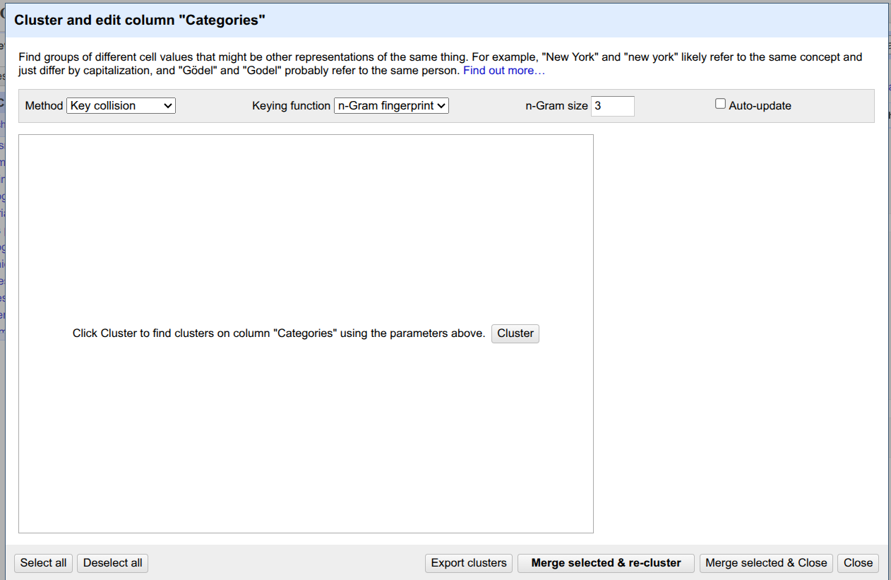
- Click on the
Clusterbutton on the left in theFacet/Filtertab.Use
Key collisionas clustering method. Change the Keying function ton-Gram fingerprintand change the n-Gram size to3.
Click on the
Clusterbutton in the middle window.
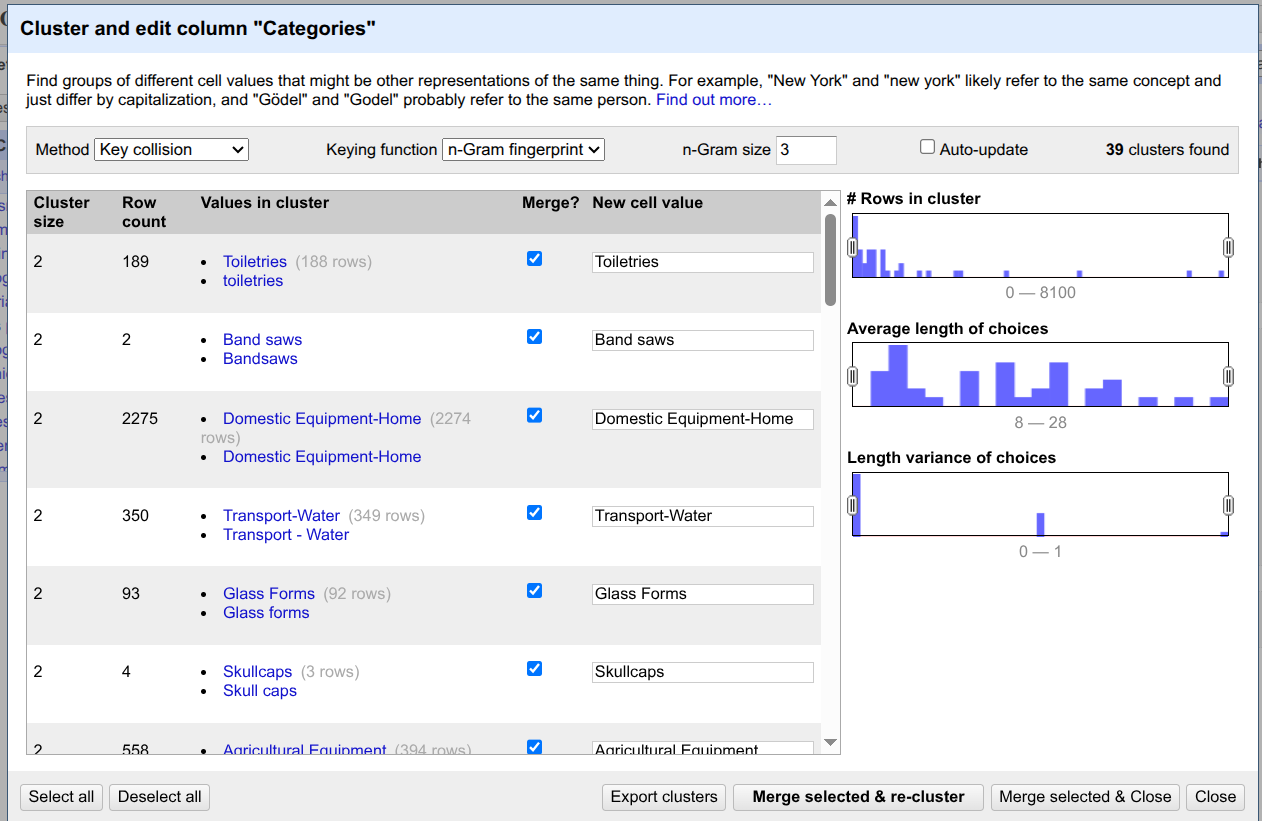
Here, you can see different suggestions from OpenRefine to cluster different categories and merge them into one. In our tutorial, we merge all the suggestions by clicking on
Select alland then clicking onMerge selected and re-cluster.Now, you can close the clustering window by clicking on
close.Be careful with clustering! Some settings are very aggressive, so you might end up clustering values that do not belong together!
Now that the different categories have been clustered individually, we can reassemble them in the respective object single cell.
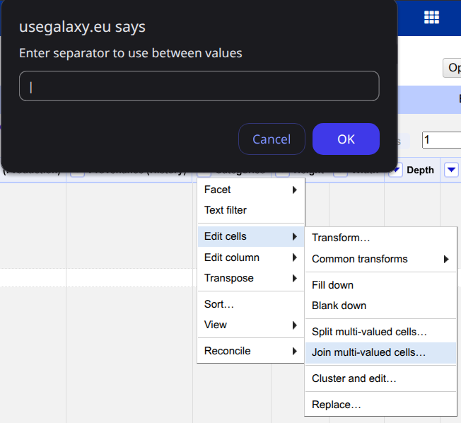
- Click the Categories triangle and hover over the
Edit cellsand click onJoin multi-valued cells.Choose the pipe character (
|) as a separator and click onOK.
The rows now look like before, with a multi-valued Categories field.
You have now successfully split, cleaned and re-joined the various categories of objects in the museum’s metadata! Congratulations. As before the splitting of columns, we are now back to 75725 rows. When you are satisfied with your data, choose whether to export the dataset to your Galaxy history or download it directly to your computer.
Exporting your data back to Galaxy
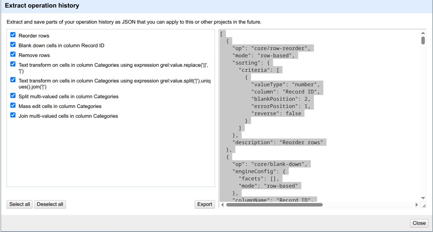
Exporting your data back to Galaxy allows you to analyse or visualise it with further tools in the platform. But OpenRefine also allows you to export your operation history, detailing all the steps you took in JSON format. This way, you can import it later and reproduce the exact same analysis. To do so:
Hands On: Exporting the OpenRefine history
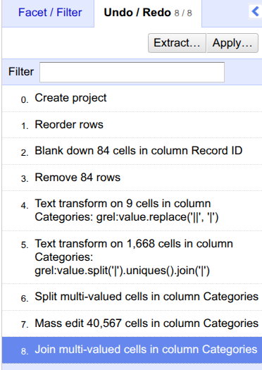
- Click on
Undo/Redoon the left panel.Click on
Extract....
- Click on the steps that you want to extract. Here, we selected everything.
- Click on
Export. Give your file a name to save it on your computer.
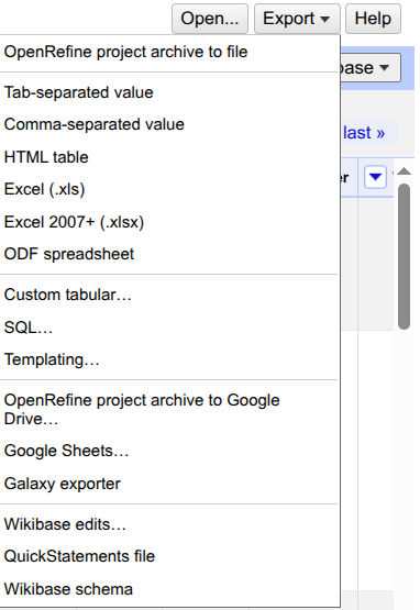
However, you will also ensure that you save your data. You can download your cleaned dataset in various formats, such as CSV, TSV, and Excel, within OpenRefine. For further analysis or visualisation, we suggest you export it to your Galaxy history.
Hands On: Exporting the results and history
- Click on
Exportat the top of the table.Select
Galaxy exporter. Wait a few seconds. In a new page, you will see a text as follows: “Dataset has been exported to Galaxy, please close this tab”. When you see this, you can close that tab.
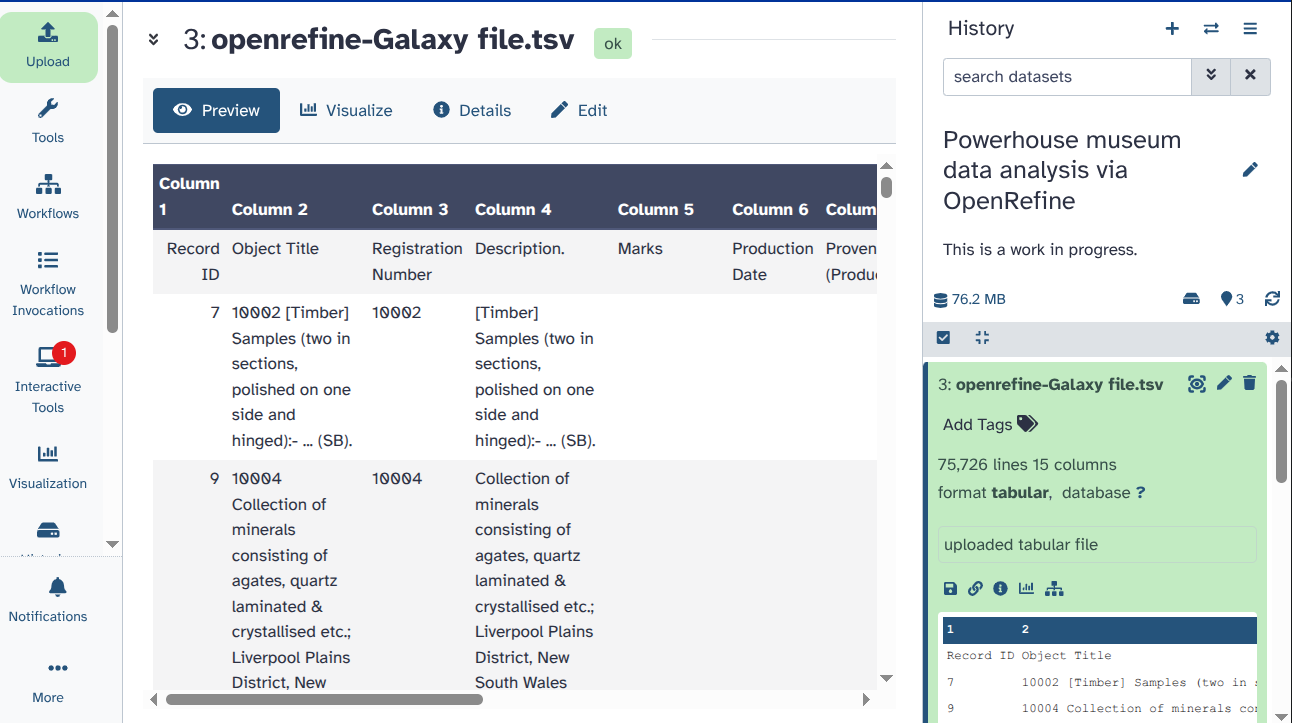
- You can now close the OpenRefine interactive tool. For that, go to your history with the orange item
OpenRefine on data [and a number]. This is your interactive tool. Click “OK” on the small square (it says “Stop this interactive tool” when you mouse over it). You do not need it for your next steps.- You can find a new dataset (named something like “openrefine-Galaxy file.tsv”) in your Galaxy History (with a green background). It contains your cleaned dataset for further analysis.
You can click on the eye icon (galaxy-eye) and investigate the table.
Awesome work! However, you may recall that we still have two unanswered questions about our data: From which year does the museum have the most objects? And what objects does the museum have from that year?
Run a Galaxy Workflow on your cleaned data
Congratulations, you have successfully cleaned your data and improved its quality! But what can you do with it now? This depends on your research objectives. For us, it is interesting to extract further information from the data. To make it easier for you, we have created a workflow that links all the tools needed for this analysis. We wanted to know which year the museum had the most objects and what they were. You can follow along and answer those questions with us, or explore the Galaxy tools on your own, to adapt the analysis to your needs. In this case, be sure to check out our other tutorials, particularly the introductory ones.
How to find and run existing workflows
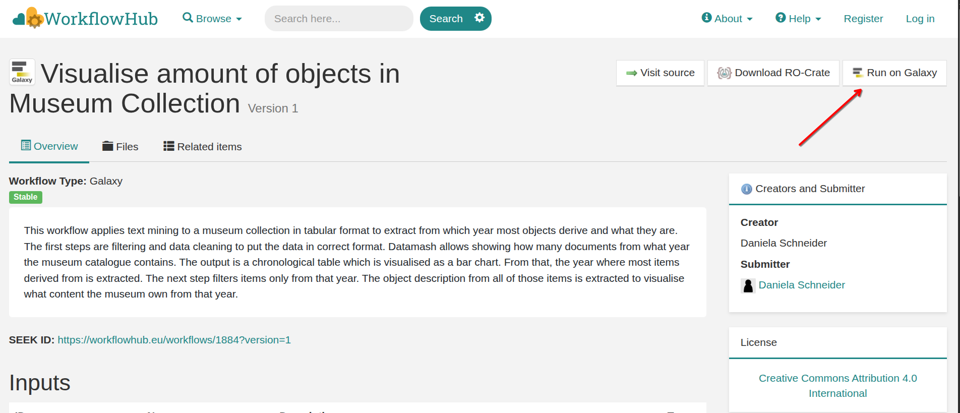
Hands On: Run a Galaxy workflow on your datasetThere are different ways to import or create a workflow to Galaxy. For example, you can import a workflow from the registered workflows on WorkflowHub which is a registry for describing, sharing, and publishing scientific computational workflows. To do that, you have to navigate to the WorkflowHub and find the workflow of interest. In this tutorial, we are working with this workflow. When you open the link to this workflow on WorkflowHub, you see the following page:
Please click on the
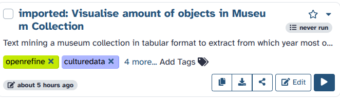
Run on Galaxybutton on top right. After doing this, you will be redirected to your Galaxy account and see the workflow automatically in your middle panel as follows:
This is one way of importing a workflow to your account.
Let’s assume you have done this and imported the workflow to your Galaxy account.
You can find all workflows available to you by clicking on the Workflows Icon (galaxy-workflows-activity) on the left panel.
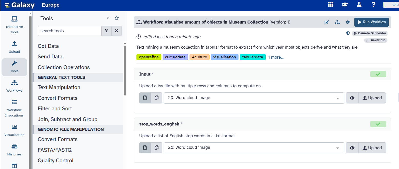
Then, you can select and run different workflows (if you have any workflows in your account). Here, let’s click on the Run button (workflow-run) of the workflow we provided to you in this tutorial.
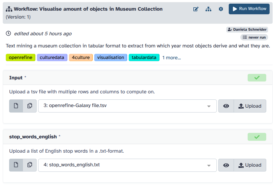
Determine the inputs as follows:
Input:
openrefine-Galaxy file.tsv—This is the file you cleaned in OpenRefine.stop_words_english:
stop_words_english.txt, which is the file we provided to you in this tutorial.
- Click on the
Run Workflowbutton at the top.You can follow the stages of different jobs (computational tasks). They will be created, scheduled, executed, and completed. When everything is green, your workflow has run fully and the results are ready.
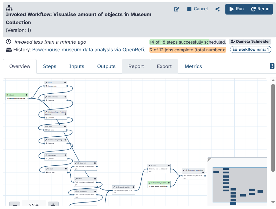
What can you see here? To follow along, we made all substeps of the task available as outputs.
To answer our question of which year most elements in the museum derive from, we first cut the column of production time from the table.
You can see this in the file Cut on Data (Number).
From this, we filter only the dates that derive from specific years, not year ranges. (See Filter Tabular on Data (Number).)
You can click on the arrow in the circle button of this dataset (Run job again) to see what exact input was used to exclude year ranges.
Regular expressions help clean remaining inconsistencies in the dataset. (Dataset: Column Regex Find And Replace on Data (Number))
Sorting the production date in descending order, as done in the dataset Sort on data (lowest Number), reveals that one faulty dataset, which is supposed to have been created in 2041, is part of the table.
We remove it in the next step with the tool Remove beginning.
The tool Datamash allows for summarising how many elements arrived at the museum in each year. (Dataset: Datamash on data (Number).)
After we apply this tool, the dataset is no longer 7738 lines long, but only 259.
This is because the number of times each year appeared in the table was summed up in a second column.
Sorting in ascending order (Sort on data (Number)) shows a chronological dataset with the earliest entries in the beginning and the most recent entries at the end of the table.
We can easily visualise this in a (particularly crowded) bar chart directly within Galaxy. (Bar chart on data (Number))
But this is not the most optimal view to show us which year most objects derive from.
To determine from which year most objects originate, we use another sorting order (Sort on Data (highest number)).
Question
- From what year does the museum have the most objects?
- The dataset
Sort on data (highest number)shows the number of objects by year, sorted from most to least. 288 items are noted for the year 1969 in the first row. This is the year from which the museum has the most (clearly datable) objects.
The next four steps parse this year as a conditional statement step by step. (Select first on data (Number), Cut on data (Number), Parse parameter value on data (Number) and Compose text parameter value.)
This means, even if you upload another dataset, the highest number is always selected and taken as an input for the next steps.
Based on this input, which is determined by the year with the highest input, Search in textfiles on data (Number) searches for object descriptions from the 288 objects of the most prominent year.
The table is very rich in information, but not that easy to digest.
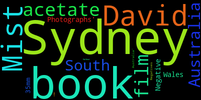
To make the table more accessible, we create a word cloud of the object descriptions with the offered stop word list.
If you click on the stop word list we provided, you see what “fill words” are excluded from the word cloud. In essence, only words conveying meaning remain.
This helps us quickly determine what kinds of objects the museum has from this popular year.
The dataset Word cloud image shows that most objects from the museum are negatives from Davis Mist, a famous Australian photographer, who created them that year and donated them to the museum.
Conclusion
Congratulations! You used OpenRefine to clean your data and ran a workflow from Galaxy with your results! You now know how to perform basic steps in Galaxy, run OpenRefine as an interactive tool, and transfer data from Galaxy to OpenRefine and back. On the way, you have learned basic data cleaning techniques, such as facetting, to enhance the quality of your data. To extract further information from the cleaned data, running a pre-designed workflow showed you a glimpse into Galaxy. Of course, you can always conduct your own analysis using the tools most useful to you, instead.
You've Finished the Tutorial
Key points
You can use OpenRefine online through Galaxy.
OpenRefine allows you to work interactively with messy data.
Galaxy allows you to run workflows with your data.
With Galaxy, you can visualise your data in various ways.
Frequently Asked Questions
Have questions about this tutorial? Have a look at the available FAQ pages and support channelsReferences
- Hooland, S. van, R. Verborgh, and M. D. Wilde, 2013 Cleaning Data with OpenRefine (A. Crymble, Ed.). Programming Historian. 10.46430/phen0023
Feedback
Did you use this material as an instructor? Feel free to give us feedback on how it went.
Did you use this material as a learner or student? Click the form below to leave feedback.

Citing this Tutorial
- Diana Chiang Jurado, Armin Dadras, Daniela Schneider, OpenRefine Tutorial for researching cultural data (Galaxy Training Materials). https://training.galaxyproject.org/training-material/topics/digital-humanities/tutorials/open-refine-tutorial/tutorial.html Online; accessed TODAY
- Hiltemann, Saskia, Rasche, Helena et al., 2023 Galaxy Training: A Powerful Framework for Teaching! PLOS Computational Biology 10.1371/journal.pcbi.1010752
- Batut et al., 2018 Community-Driven Data Analysis Training for Biology Cell Systems 10.1016/j.cels.2018.05.012
@misc{digital-humanities-open-refine-tutorial,
author = "Diana Chiang Jurado and Armin Dadras and Daniela Schneider",
	title = "OpenRefine Tutorial for researching cultural data (Galaxy Training Materials)",
	year = "",
	month = "",
	day = "",
	url = "\url{https://training.galaxyproject.org/training-material/topics/digital-humanities/tutorials/open-refine-tutorial/tutorial.html}",
	note = "[Online; accessed TODAY]"
}
@article{Hiltemann_2023,
	doi = {10.1371/journal.pcbi.1010752},
	url = {https://doi.org/10.1371%2Fjournal.pcbi.1010752},
	year = 2023,
	month = {jan},
	publisher = {Public Library of Science ({PLoS})},
	volume = {19},
	number = {1},
	pages = {e1010752},
	author = {Saskia Hiltemann and Helena Rasche and Simon Gladman and Hans-Rudolf Hotz and Delphine Larivi{\`{e}}re and Daniel Blankenberg and Pratik D. Jagtap and Thomas Wollmann and Anthony Bretaudeau and Nadia Gou{\'{e}} and Timothy J. Griffin and Coline Royaux and Yvan Le Bras and Subina Mehta and Anna Syme and Frederik Coppens and Bert Droesbeke and Nicola Soranzo and Wendi Bacon and Fotis Psomopoulos and Crist{\'{o}}bal Gallardo-Alba and John Davis and Melanie Christine Föll and Matthias Fahrner and Maria A. Doyle and Beatriz Serrano-Solano and Anne Claire Fouilloux and Peter van Heusden and Wolfgang Maier and Dave Clements and Florian Heyl and Björn Grüning and B{\'{e}}r{\'{e}}nice Batut and},
	editor = {Francis Ouellette},
	title = {Galaxy Training: A powerful framework for teaching!},
	journal = {PLoS Comput Biol}
}
Funding
These individuals or organisations provided funding support for the development of this resource
Congratulations on successfully completing this tutorial!You can use Ephemeris's
shed-tools installcommand to install the tools used in this tutorial.shed-tools install [-g GALAXY] [-a API_KEY] -t <(curl https://training.galaxyproject.org/training-material/api/topics/digital-humanities/tutorials/open-refine-tutorial/tutorial.json | jq .admin_install_yaml -r)Alternatively you can copy and paste the following YAML
---
install_tool_dependencies: true
install_repository_dependencies: true
install_resolver_dependencies: true
tools:
- name: text_processing
  owner: bgruening
  revisions: ab83aa685821
  tool_panel_section_label: Text Manipulation
  tool_shed_url: https://toolshed.g2.bx.psu.edu/
- name: text_processing
  owner: bgruening
  revisions: ab83aa685821
  tool_panel_section_label: Text Manipulation
  tool_shed_url: https://toolshed.g2.bx.psu.edu/
- name: text_processing
  owner: bgruening
  revisions: ab83aa685821
  tool_panel_section_label: Text Manipulation
  tool_shed_url: https://toolshed.g2.bx.psu.edu/
- name: wordcloud
  owner: bgruening
  revisions: 45c4cc885ddb
  tool_panel_section_label: Graph/Display Data
  tool_shed_url: https://toolshed.g2.bx.psu.edu/
- name: regex_find_replace
  owner: galaxyp
  revisions: 503bcd6ebe4b
  tool_panel_section_label: Text Manipulation
  tool_shed_url: https://toolshed.g2.bx.psu.edu/
- name: compose_text_param
  owner: iuc
  revisions: e188c9826e0f
  tool_panel_section_label: Expression Tools
  tool_shed_url: https://toolshed.g2.bx.psu.edu/
- name: datamash_ops
  owner: iuc
  revisions: aaafc0ac4dd2
  tool_panel_section_label: Join, Subtract and Group
  tool_shed_url: https://toolshed.g2.bx.psu.edu/
- name: filter_tabular
  owner: iuc
  revisions: 90f657745fea
  tool_panel_section_label: Text Manipulation
  tool_shed_url: https://toolshed.g2.bx.psu.edu/