Visualization of Climate Data using NetCDF xarray Map Plotting
| Author(s) |
|
| Reviewers |
|
OverviewQuestions:
Objectives:
What is xarray map plotting?
How to plot NetCDF data using xarray map plotting tool?
What are the different types of projections and colormap options available in the tool?
Requirements:
Learn about plotting Climate Data
Learn about NetCDF xarray map plotting tool
Learn about visualizing the climate data using NetCDF xarray map plotting using the different kinds of projections and colormap options
Time estimation: 1 hourLevel: Introductory IntroductorySupporting Materials:Published: Oct 26, 2022Last modification: Jun 27, 2024License: Tutorial Content is licensed under Creative Commons Attribution 4.0 International License. The GTN Framework is licensed under MITpurl PURL: https://gxy.io/GTN:T00136version Revision: 9
The data used in this tutorial is ECMWF Reanalysis 5 hourly data on single levels. We are interested in the following variables: air temperature at 2 metres, latitude, longitude and time. Our main objective is to plot the global air temperature at 2 metres with respect to time. For this we will be using the netCDF xarray tool available in the Galaxy Europe (or your favourite Galaxy Instance) server.
It will be a fun learning experience for anyone who loves visualization !
CommentThe tutorial aims for establishing a good knowledge about meaningful visualization of climate data.
It is beginner friendly and does not require much knowledge about the tool.
AgendaIn this tutorial we will deal with:
Comment: BackgroundAccording to UN , Climate is the long term shift in temperature and weather patterns which may be due to natural or artificial causes. To learn more about climate, refer this tutorial from the GTN. Due to the frequently changing nature of the weather patterns, the size of the collected data is huge. The climate data is mainly represented in these three categories : NetCDF (Network Common Data Form), HDF (Hierarchical Data Format) , GRIB (GRIdded Binary or General Regularly-distributed Information in Binary form).
The NetCDF file format is basically used for storing multidimensional data which generally consists of variables such as temperature, precipitation, wind direction, etc. The variation of climate variables over a period of time is suitably plotted using this dataset. The entire earth is divided into both horizontal as well as vertical coordinates which makes plotting of the variables such as the ocean temperatures possible.
The coordinate system, types of projections and colormaps are some of the very important considerations in achieving the most suitable visualization option.
Get data
Hands On: Data upload
Create a new history for this tutorial. Name it as per your choice. My suggestions : ECMWF_Reanalysis.
To create a new history simply click the new-history icon at the top of the history panel:
- Import remote files
- location:
ECMWF ERA5 Reanalysis->2022->05->data->air_temperature_at_2_metres.ncAs an alternative to uploading the data from a URL or your computer, the files may also have been made available from a Choose from repositories:
- Click on Upload Data on the top of the left panel
Click on Choose from repository and scroll down to find your repository or type the repository name in the
search boxon the top.
- Look for your data under:
ECMWF ERA4 Reanalysis -> 2022 -> 05 -> data -> air_temperature_at_2_metres.nc- Select the datasets you want to import
- click on OK
- Click on Start
- Click on Close
- You can find the dataset has begun loading in you history.
or, if this is not available, you can import from Zenodo:
https://zenodo.org/record/6621460/files/air_temperature_at_2_metres.netcdf
- Copy the link location
Click galaxy-upload Upload at the top of the activity panel
- Select galaxy-wf-edit Paste/Fetch Data
Paste the link(s) into the text field
Press Start
- Close the window
- Check the datatype of uploaded data, it should be
netCDF.
- If it is not
netCDF, make sure to convert it using the Galaxy built-in format converters.
- Click on the galaxy-pencil pencil icon for the dataset to edit its attributes.
- In the central panel, click galaxy-chart-select-data Datatypes tab on the top.
- In the galaxy-gear Convert to Datatype section, select
Convert h5 to netCDFfrom “Target datatype” dropdown.- Click the Create Dataset button to start the conversion.
Rename Datasets galaxy-pencil if you find the name to be too long or you have something more meaningful in your mind.
Tag Datasets galaxy-tags with the tag
#ecmwfDatasets can be tagged. This simplifies the tracking of datasets across the Galaxy interface. Tags can contain any combination of letters or numbers but cannot contain spaces.
To tag a dataset:
- Click on the dataset to expand it
- Click on Add Tags galaxy-tags
- Add tag text. Tags starting with
#will be automatically propagated to the outputs of tools using this dataset (see below).- Press Enter
- Check that the tag appears below the dataset name
Tags beginning with
#are special!They are called Name tags. The unique feature of these tags is that they propagate: if a dataset is labelled with a name tag, all derivatives (children) of this dataset will automatically inherit this tag (see below). The figure below explains why this is so useful. Consider the following analysis (numbers in parenthesis correspond to dataset numbers in the figure below):
- a set of forward and reverse reads (datasets 1 and 2) is mapped against a reference using Bowtie2 generating dataset 3;
- dataset 3 is used to calculate read coverage using BedTools Genome Coverage separately for
+and-strands. This generates two datasets (4 and 5 for plus and minus, respectively);- datasets 4 and 5 are used as inputs to Macs2 broadCall datasets generating datasets 6 and 8;
- datasets 6 and 8 are intersected with coordinates of genes (dataset 9) using BedTools Intersect generating datasets 10 and 11.
Now consider that this analysis is done without name tags. This is shown on the left side of the figure. It is hard to trace which datasets contain “plus” data versus “minus” data. For example, does dataset 10 contain “plus” data or “minus” data? Probably “minus” but are you sure? In the case of a small history like the one shown here, it is possible to trace this manually but as the size of a history grows it will become very challenging.
The right side of the figure shows exactly the same analysis, but using name tags. When the analysis was conducted datasets 4 and 5 were tagged with
#plusand#minus, respectively. When they were used as inputs to Macs2 resulting datasets 6 and 8 automatically inherited them and so on… As a result it is straightforward to trace both branches (plus and minus) of this analysis.More information is in a dedicated #nametag tutorial.


What is xarray?
xarray, formerly known as xray, is a python package which enables us to play with gridded data. This package shares most of its features from numpy, but in a more convenient manner by keeping track of labels in arrays. The gridded data is mainly available in netCDF data format. Thus xarray comes very handy while dealing with netCDF files.
What is Visualisation in xarray?
xarray uses Cartopy and Matplotlib as the two main tools for creating detailed and informative plots. Cartopy is a python package used for geospatial data analysis. In the Python library, matplotlib is the most used scientific plotting library. For a multidimensional data consisting of latitudes and longitudes along with the other variables, xarray has the capability of appling cartopy map projections.
Splitting the dataset using seltimestep, splithour and plotting
After loading the required data, the following stage is to obtain the meta info or meta data of the file. The very purpose of these steps are to obtain the information about dimensions, variables, global attributes, etc. The coordinate info helps to know about the actual data entries present under the various variables.
Follow the below steps:
NetCDF xarray Metadata Info
Hands On: netCDF dataset with xarray metadata Galaxy Tool
- In the tools search for NetCDF xarray Metadata Info ( Galaxy version 0.15.1) with the following parameter:
- param-file “Netcdf file”:
air_temperature_at_2_metres.ncand click onExecute.- View galaxy-eye the two generated outputs:
Metadata infosis atabularproviding the list of variables, their dimension names and number of elements per dimension. This file is used by other xarray Tools.- The second file
info fileprovides a summary of the xarray Dataset contained in your netCDF file.
Question
- What is the name of the variable for air temperature at 2 metres. What are its physical units?
- Information about variable names and units can be found in info file that was generated by xarray metadata Galaxy Tool.
- Variable name:
air_temperature_at_2_metres- Units:
KCode Outxarray.Dataset { dimensions: lat = 721 ; lon = 1440 ; time0 = 595 ; variables: float32 lon(lon) ; lon:standard_name = longitude ; lon:long_name = longitude ; lon:units = degrees_east ; float32 lat(lat) ; lat:standard_name = latitude ; lat:long_name = latitude ; lat:units = degrees_north ; datetime64[ns] time0(time0) ; time0:standard_name = time ; float32 air_temperature_at_2_metres(time0, lat, lon) ; air_temperature_at_2_metres:standard_name = air_temperature ; air_temperature_at_2_metres:units = K ; air_temperature_at_2_metres:long_name = 2 metre temperature ; air_temperature_at_2_metres:nameECMWF = 2 metre temperature ; air_temperature_at_2_metres:shortNameECMWF = 2t ; air_temperature_at_2_metres:nameCDM = 2_metre_temperature_surface; air_temperature_at_2_metres:product_type = analysis ; // global attributes: :source = Reanalysis ; :institution = ECMWF ; :title = ERA5 forecasts ; }
Sub-step with NetCDF xarray Coordinate Info
Hands On: Get Coordinate information with xarray Coordinate
- NetCDF xarray Coordinate Info ( Galaxy version 0.20.2+galaxy0) with the following parameters:
- param-file “Netcdf file”:
air_temperature_at_2_metres.nc.- View galaxy-eye the 4 generated outputs:
lat: a tabular file containing all the latitude values of our Xarray dataset;lon: a tabular file containing all the longitudes values;time0: this tabular file contains all the times extracted from the netCDF file. In our case, these are relative to 01/05/2022, 00:00:00 UTC;version: this is a text file returning the xarray package version. It is useful when publishing your Galaxy workflow.
CommentThe number of tabular files returned by this programme is proportional to the number of coordinate variables in your input file. No further processing is done after decoding the values from the netCDF input file. As a result, depending on how the original input file was coded, units for latitudes, longitudes, (level, if this dimension was present, which is not the case in this particular case) and time may differ from one file to the next.
Question: Understanding air temperature coordinates at 2 metres
- What is the format of time coordinate?
- What is the range of values for latitude and longitude?
- The
info filetells us thattime0is coded astimedelta64[ns]i.e. the time differences are in ns (here in nanoseconds). The format of time isyy-mm-dd hh:mm:ss. If we look at the tabular file namedtime0(generated byNetCDF xarray Coordinate Info), we see that these times are automatically converted to human readable time format when printed:Code Out0 2022-05-01 00:00:00 1 2022-05-01 01:00:00 2 2022-05-01 02:00:00 3 2022-05-01 03:00:00 4 2022-05-01 04:00:00This tells us that we have hourly forecast data.
2.If we look at the tabular file named
latandlon(generated byNetCDF xarray Coordinate Info), we see that these files are displayed with two columns e.g. index numbers and corresponding values. From these, we infer that the range of values forlatis90.0to-90.0and forlonis0to359.75.
Operations on Climate data using CDO Operations
We have hourly data. In order to plot it, we must first extract the hours from the bigger dataset. This is done using the seltimestep and the splithour options available in the CDO Operations tool. splithour is used when we wish to plot more than an hour. Our main aim is to plot the last hour data on the last day present in the dataset.
Hands On: Defining a particular time range using seltimestep
- CDO Operations ( Galaxy version 2.0.0+galaxy0) with the following parameters:
- In “CDO Operators”:
- param-repeat “Insert CDO Operators”
- “Select cdo operator”:
seltimestep (Select timesteps)- “Timesteps for selection”:
744/744- param-file “Additional input file”:
air_temperatures_at_2_metres.ncCommentThe syntax of using the
seltimestepis(initial data number / final data entry). An important thing to pay attention to is how the data entries are numbered: are they numbered starting from 0 or 1. Accordingly we can add or skip adding 1 to the data number to achieve the desired result.Although we are not using
splithourhere, you can find below the syntax for future uses.
CDO Operations ( Galaxy version 2.0.0+galaxy0) with the following parameters:
- In “CDO Operators”:
- param-repeat “Insert CDO Operators”
- “Select cdo operator”:
splithour (Split hours)- param-file “Additional input file”:
outfile.netcdfgenerated from the previous step.This step generates that
Nnumber ofoutfiles.netcdffiles whereNis the range of selection. Suppose your selected range was744/744for theseltimestep, then it will generate2files which can be plotted further.
Finding the NetCDF xarray Metadata Info
Hands On: netCDF dataset with xarray metadata Galaxy Tool for the hourly plots
- NetCDF xarray Metadata Info ( Galaxy version 0.15.1) with the following parameters:
- param-file “Netcdf file”:
outfile.netcdf. .- View galaxy-eye the two generated outputs:
Metadata infosis atabularproviding the list of variables, their dimension names and number of elements per dimension. This file is used by other xarray Tools.- The second file
info fileprovide a summary of the xarray Dataset contained in your netCDF file.
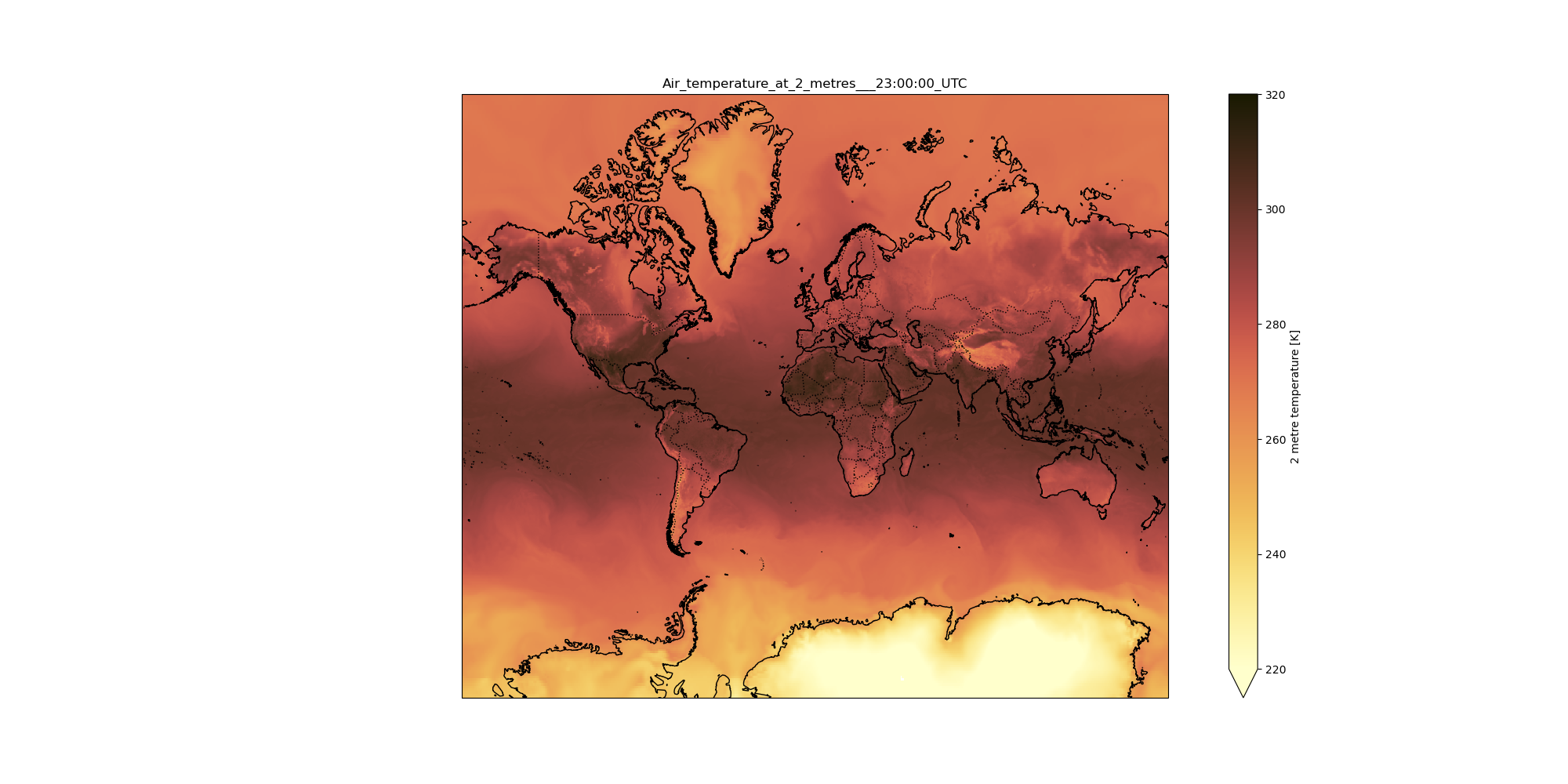
Map Plotting using NetCDF xarray map plotting
Hands On: Plotting the data of the last hour of the dayThe air temperatures corresponding to the 744th time step from the original netCDF file, namely
23:00:00for 31st May 2022 is plotted here :
- NetCDF xarray map plotting ( Galaxy version 0.20.2+galaxy0) with the following parameters:
- param-file “Netcdf file”:
outfile.netcdf- param-file “Tabular of variables”:
Metadata infos from outfile.netcdf(output of NetCDF xarray Metadata Info >tool)- “Choose the variable to plot”:
air_temperature_at_2_metres- “Name of latitude coordinate”:
lat- “Name of longitude coordinate”:
lon- “Datetime selection”:
No- “Range of values for plotting e.g. minimum value and maximum value (minval,maxval) (optional)”:
220,320- “Add country borders with alpha value [0-1] (optional)”:
1.0- “Add coastline with alpha value [0-1] (optional)”:
1.0- “Add ocean with alpha value [0-1] (optional)”:
1.0- “Specify plot title (optional)”:
Air_temperature_at_2_metres___23:00:00_UTC- “Specify which colormap to use for plotting (optional)”:
lajolla- “Specify the projection (proj4) on which we draw e.g. {“proj”:”PlateCarree”} with double quote (optional)”:
{'proj': 'Mercator'}
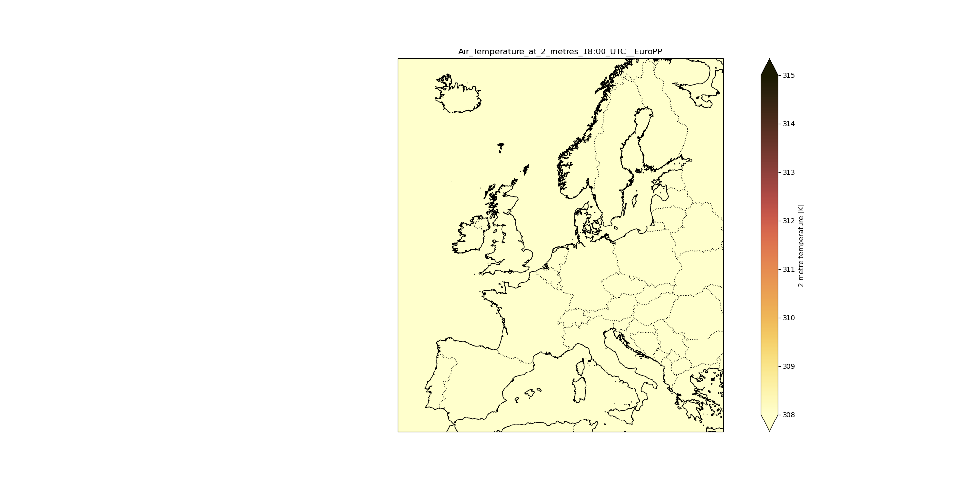
Xarray Map Plotting comes with a variety of projections. There are basically four types of projections available namely Azimuthal, Conic, Cylindrical and Pseudo-cylindrical.
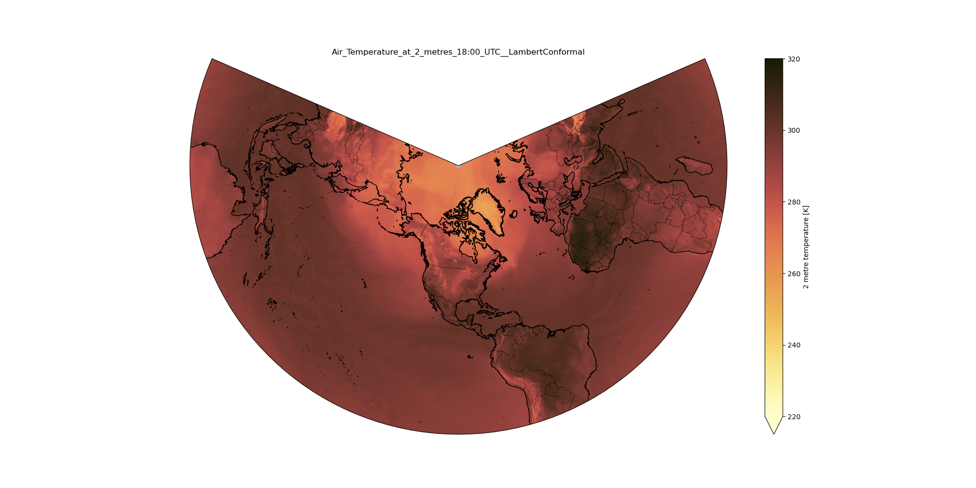
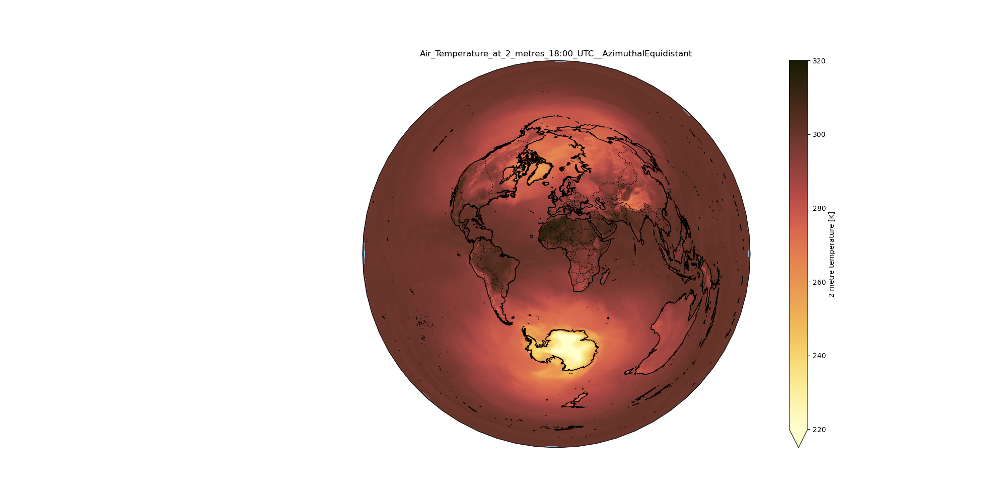
The Azimuthal projection depicts the surface of the earth with the help of a flat plane. It is also known as ‘Plane Projection.’ This simple projection type forms a family of projections by considering the poles in “normal aspect.” Another form of this projection is Azimuthal Equidistant Projection. It preserves both directions and distance from the central point of the earth. The stereographic projection which is a type of azimuthal projection was created before 150AD and deployed while mapping areas over the poles. The conic type is based on the concept of projecting the surface of the Earth on a conical surface which is unrolled into a plane surfaced map. Some of the examples of conic type of projections are : Albers Equal Area Conic, Equidistant Conic, Lambert Conformal Conic, and Polyconic. This type of projection basically has a big implementation in aviation navigation.
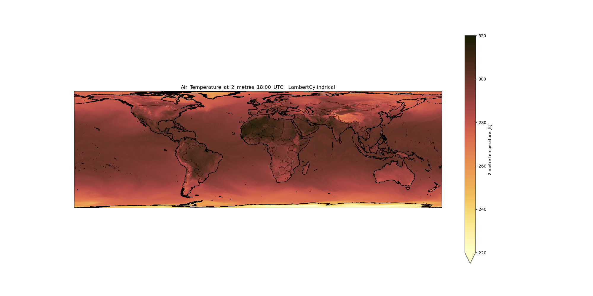
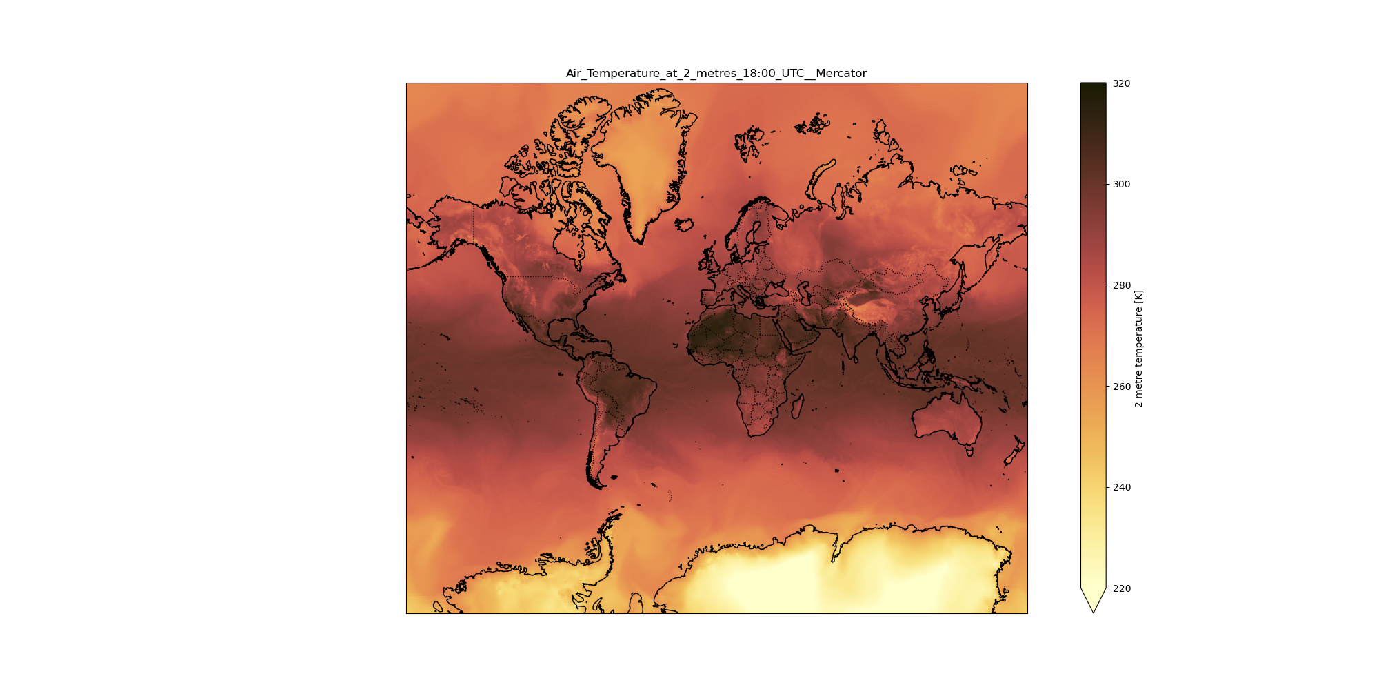
The cylindrical type is based on the concept of plotting the geographical features on the surface of the cylinder and then it is unrolled to present as a flat projection. Some examples of cylindrical projections are : Cylindrical Equal Area, Behrmann Cylindrical Equal-Area , Stereographic Cylindrical, Peters, Mercator, and Transverse Mercator. Mercator is one of the most famous and preferred type of projection. The straight lines (Rhumb Lines) are best for the navigation process.
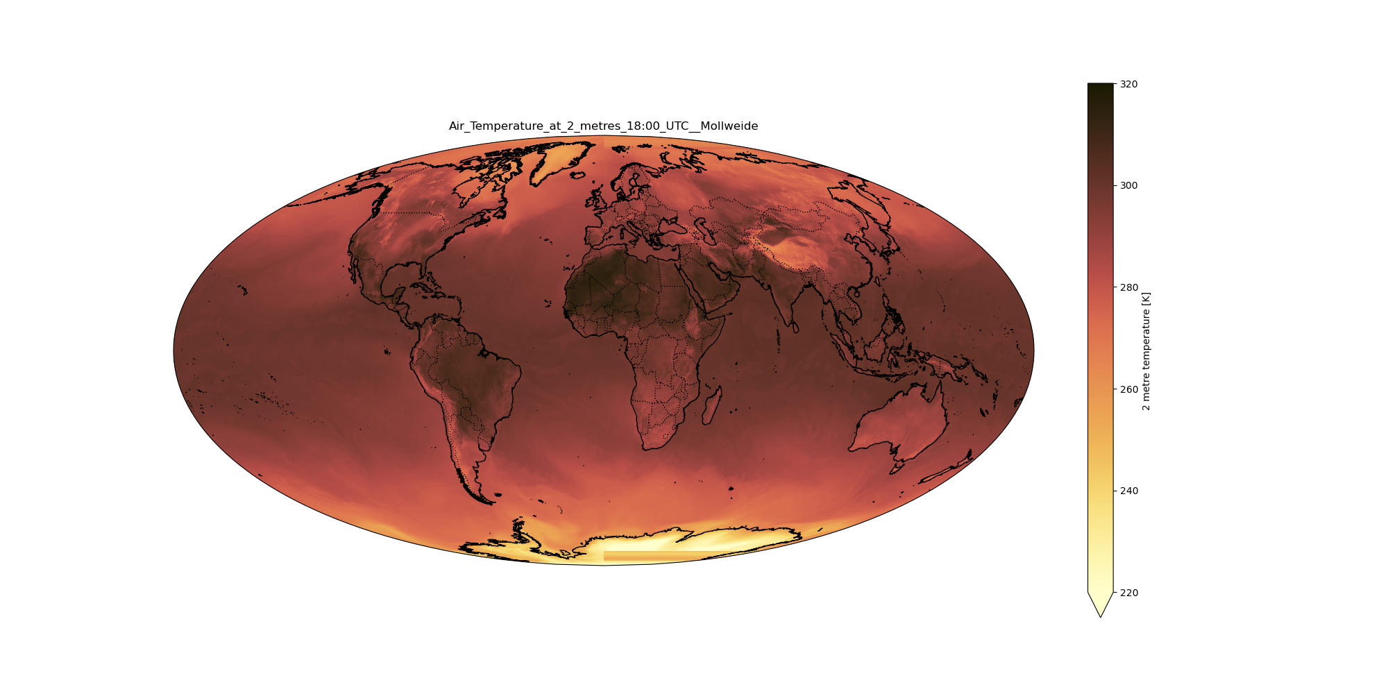
In the pseudo cylindrical type of projection , the meridians are straight instead of being curved. These kinds of projections are characterised by straight horizontal lines for parallels of latitude and (usually) equally-spaced curved meridians of longitude. Oval projections pinched or flattened at the poles are its identifying features.
Projections:
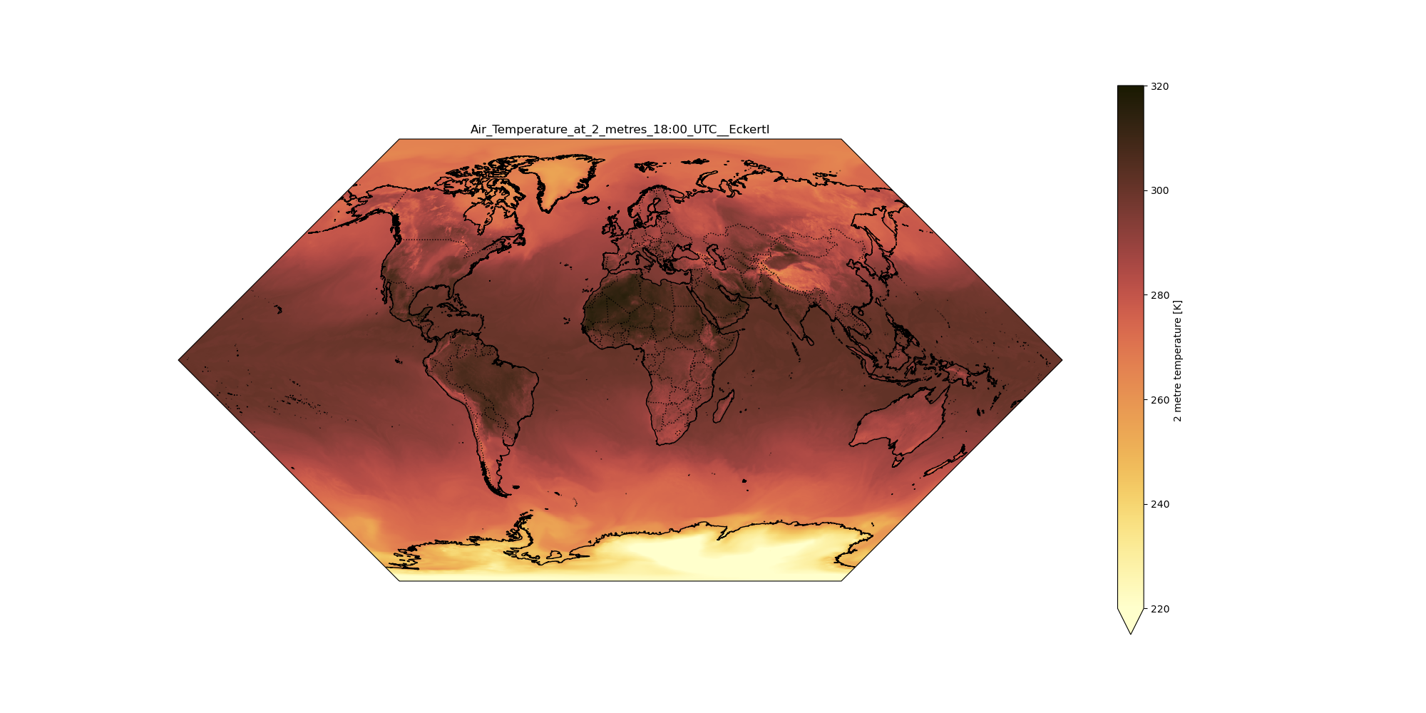
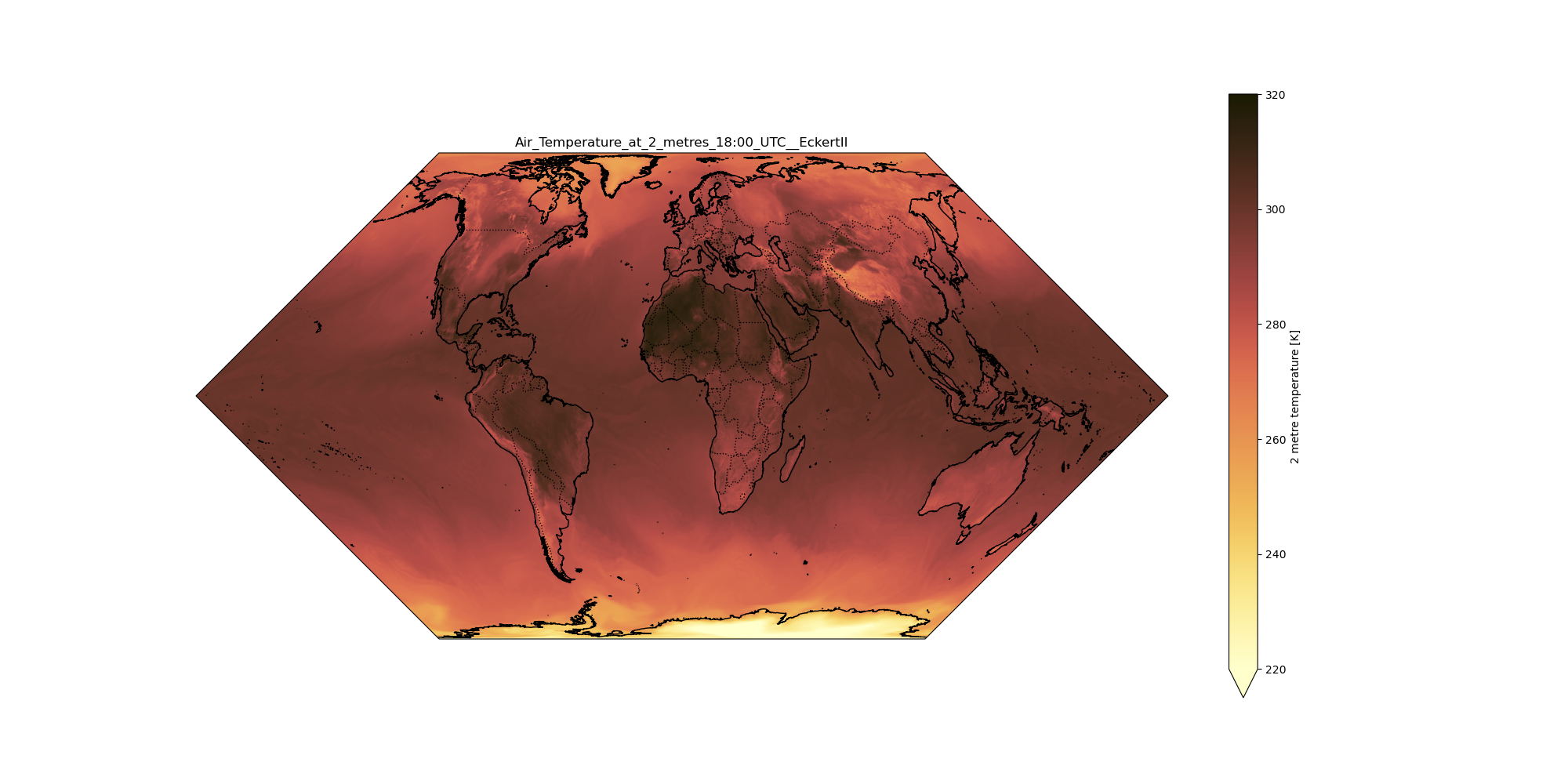
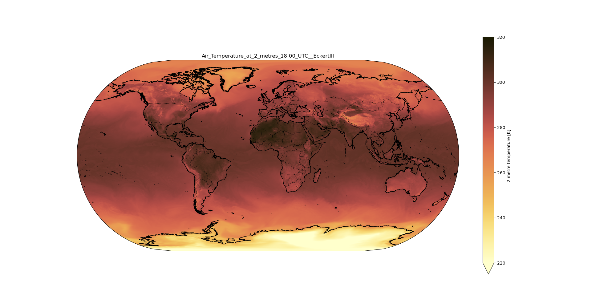
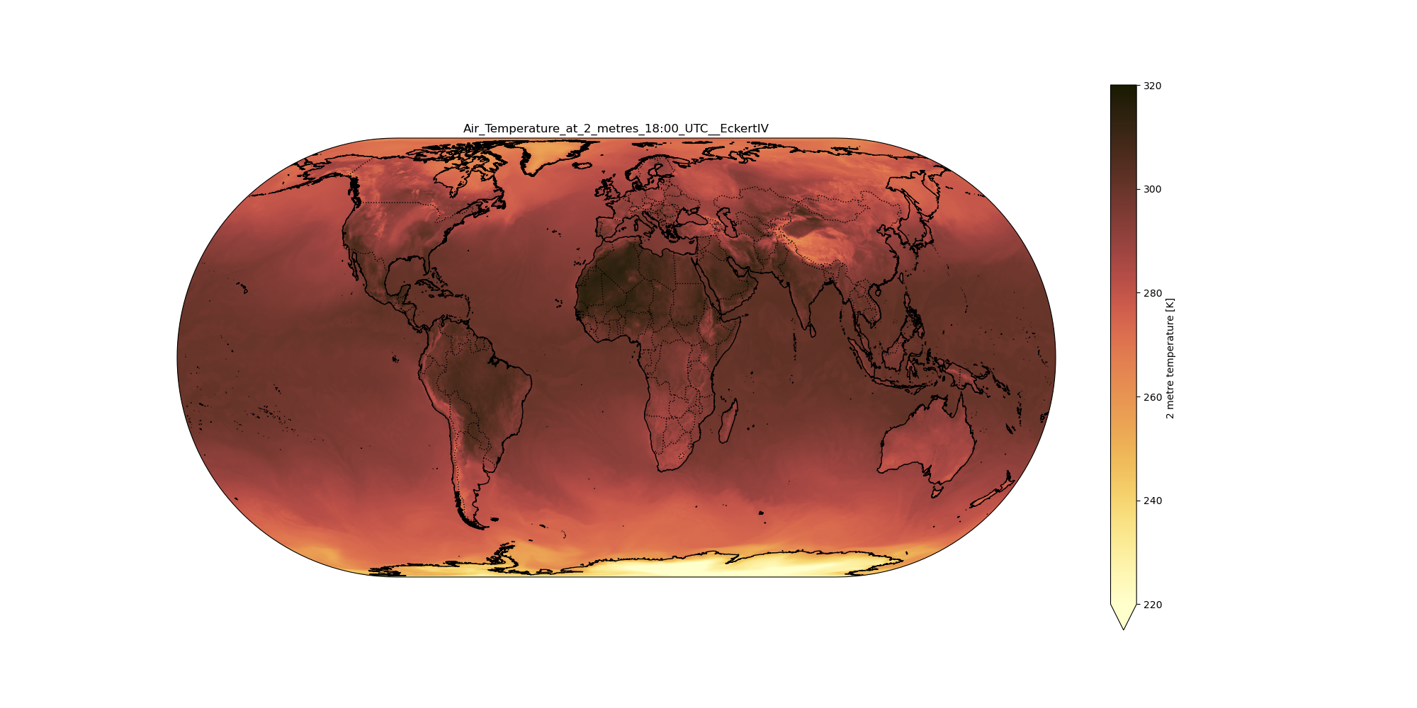
There are about 30 different kinds of projections available in the proj option. The basic knowledge of projections is very essential in plotting out the best fit map. Below is the list of plots deployed using the various kinds of projections supported by the NetCDF xarray mapplotting tool.
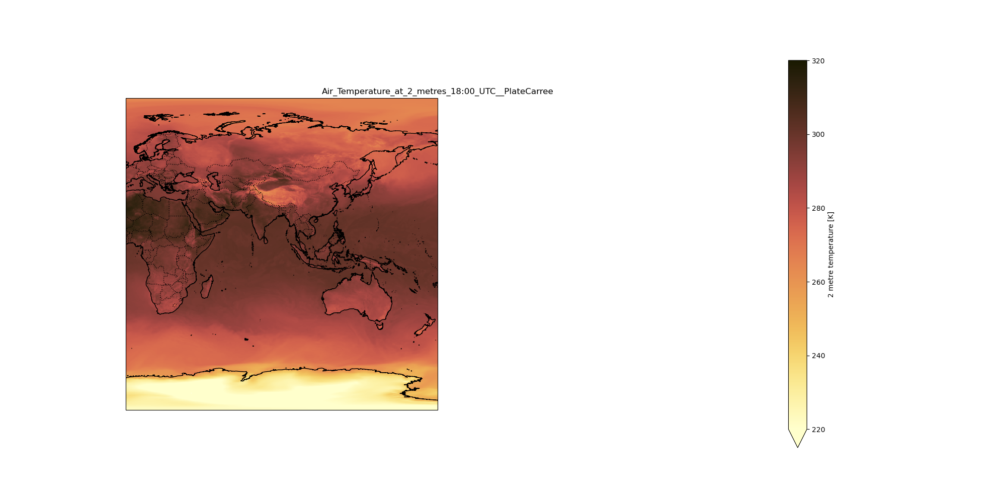
PlateCarree Syntax: {“proj”:”PlateCarree”}
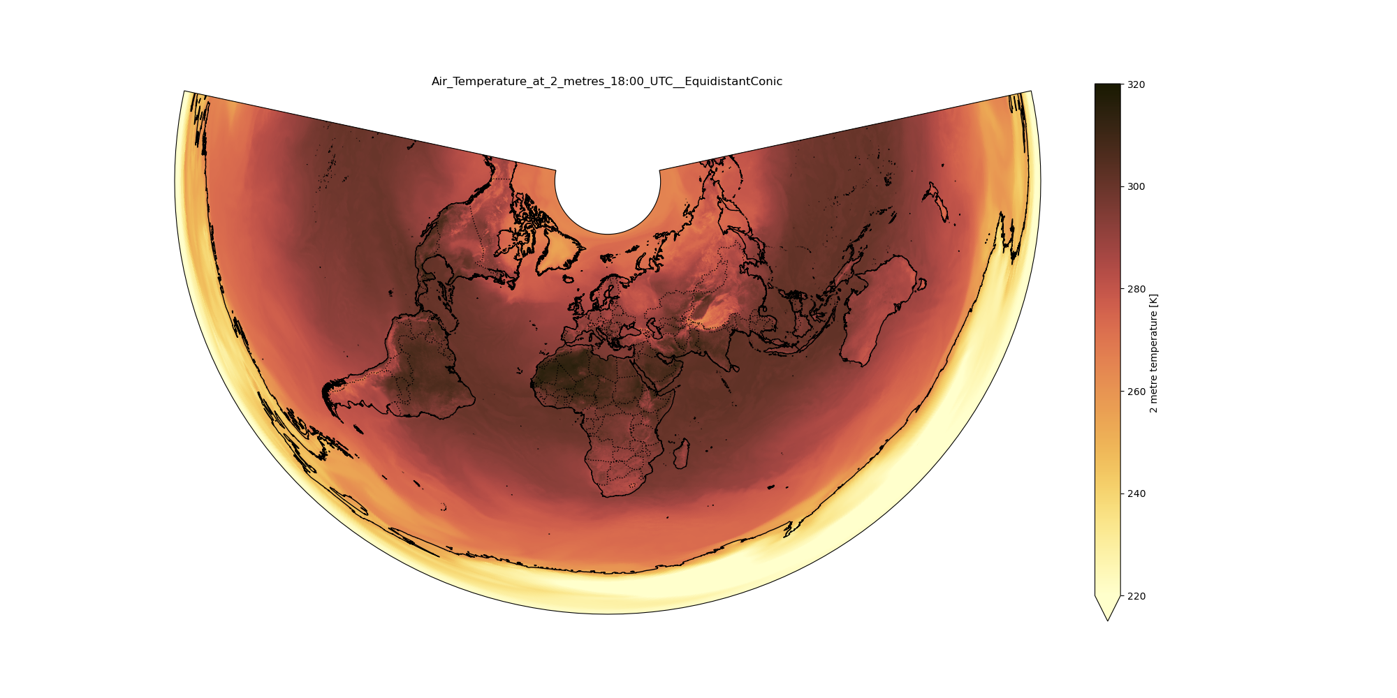
EquidistantConic Syntax: {“proj”:”EquidistantConic”, “central_longitude”: 20.0, “central_latitude”: 70.0 }
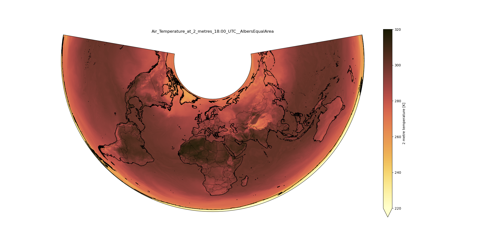
AlbersEqualArea Syntax: {“proj”:”AlbersEqualArea”, “central_longitude”: 20.0, “central_latitude”: 70.0 }
EuroPP Syntax: {“proj”:”EuroPP”}
LambertConformal Syntax:{“proj”:”LambertConformal” }
AzimuthalEquidistant Syntax: {“proj”:”AzimuthalEquidistant” }
LambertCylindrical Syntax:{“proj”:”LambertCylindrical”}
Mercator Syntax: {“proj”:”Mercator” }
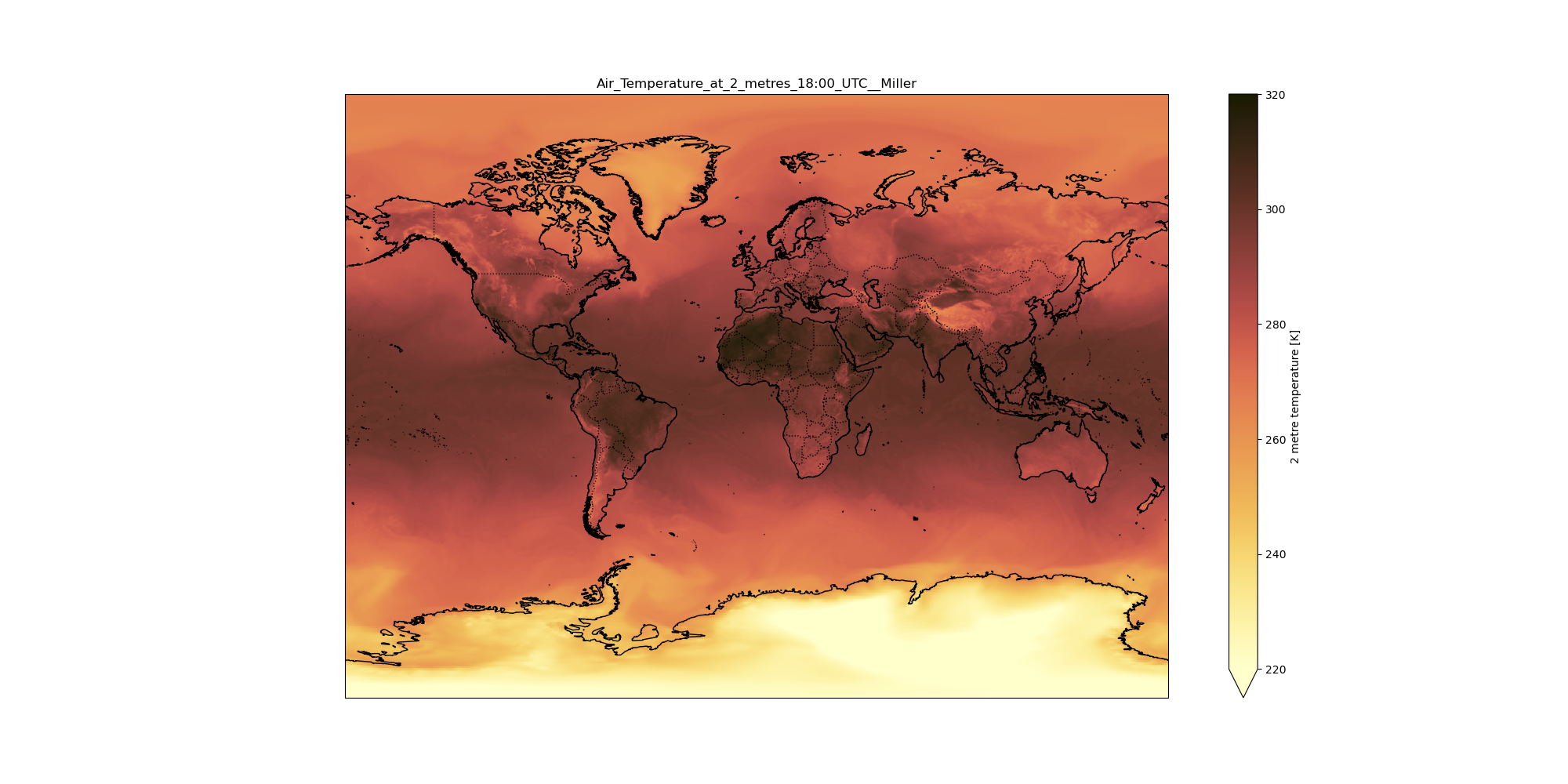
Miller Syntax: {“proj”:”Miller” }
Mollweide Syntax: {“proj”:”Mollweide” }
Orthographic Syntax:{“proj”:”Orthographic” }
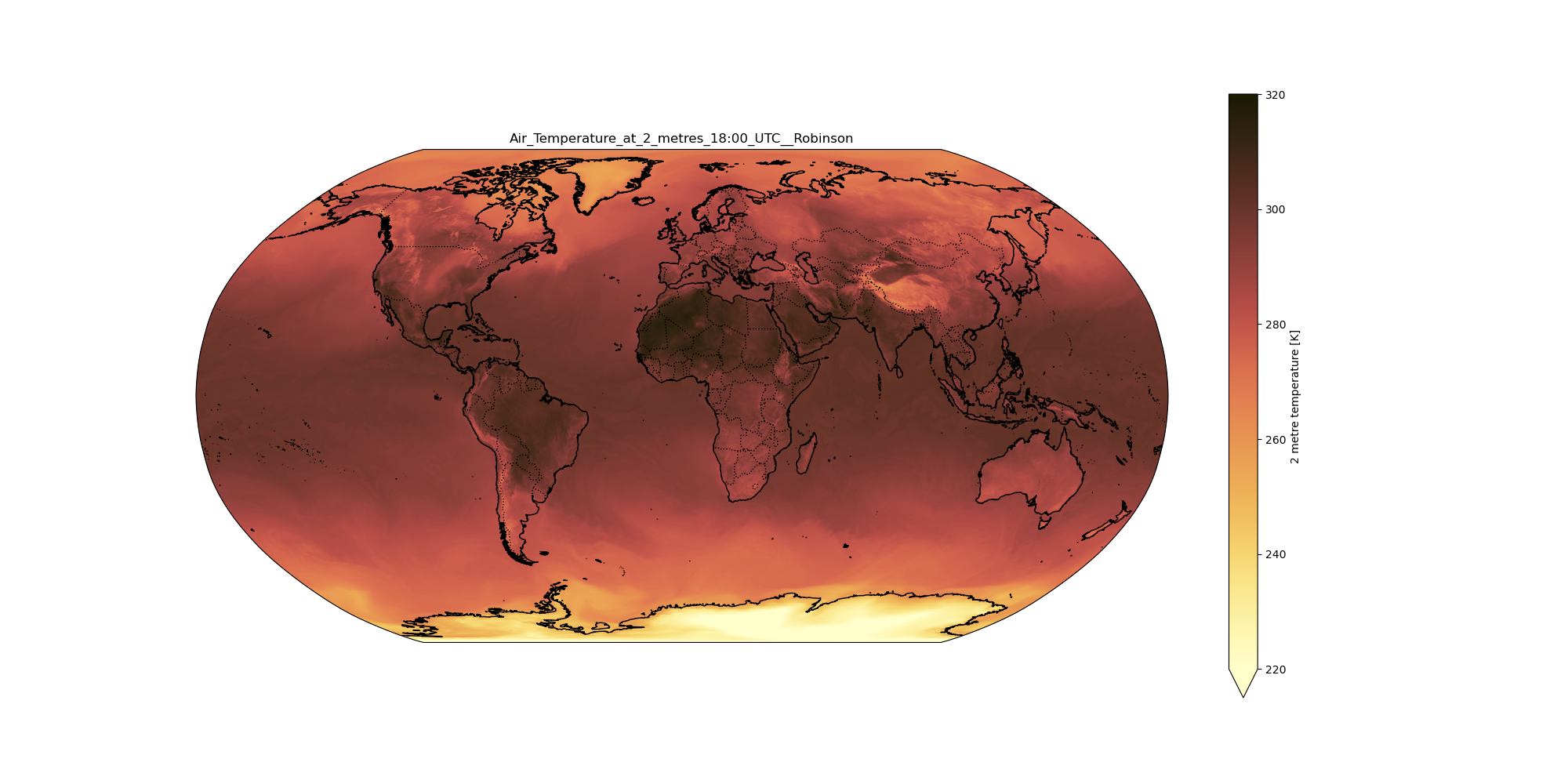
Robinson Syntax: {“proj”:”Robinson” }
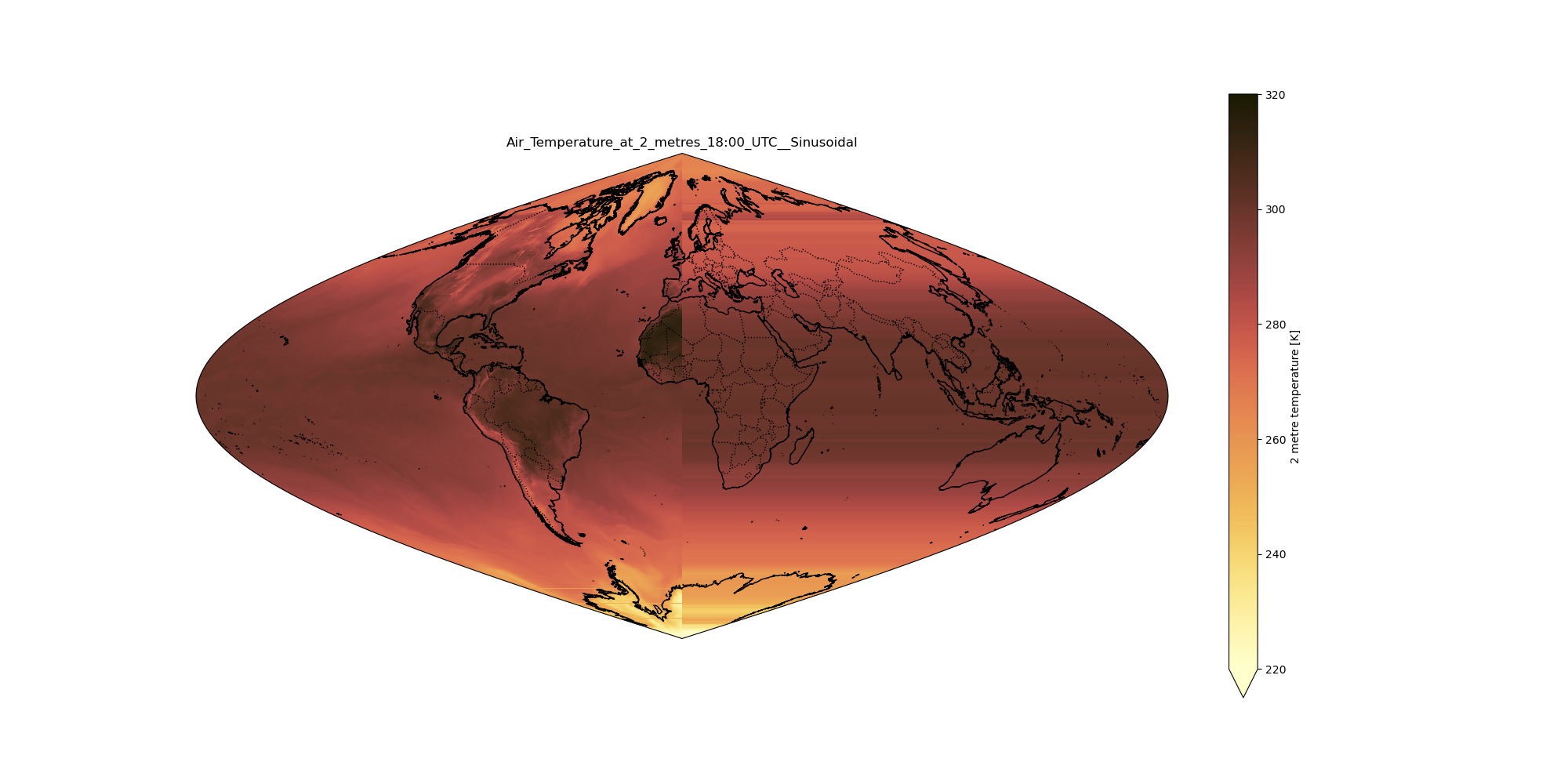
Sinusoidal Syntax: {“proj”:”Sinusoidal” }
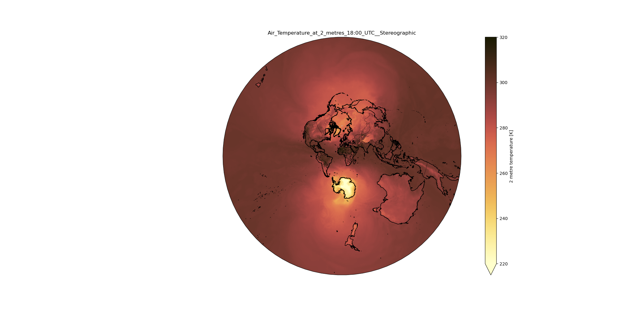
Stereographic Syntax: {“proj”:”Stereographic” }
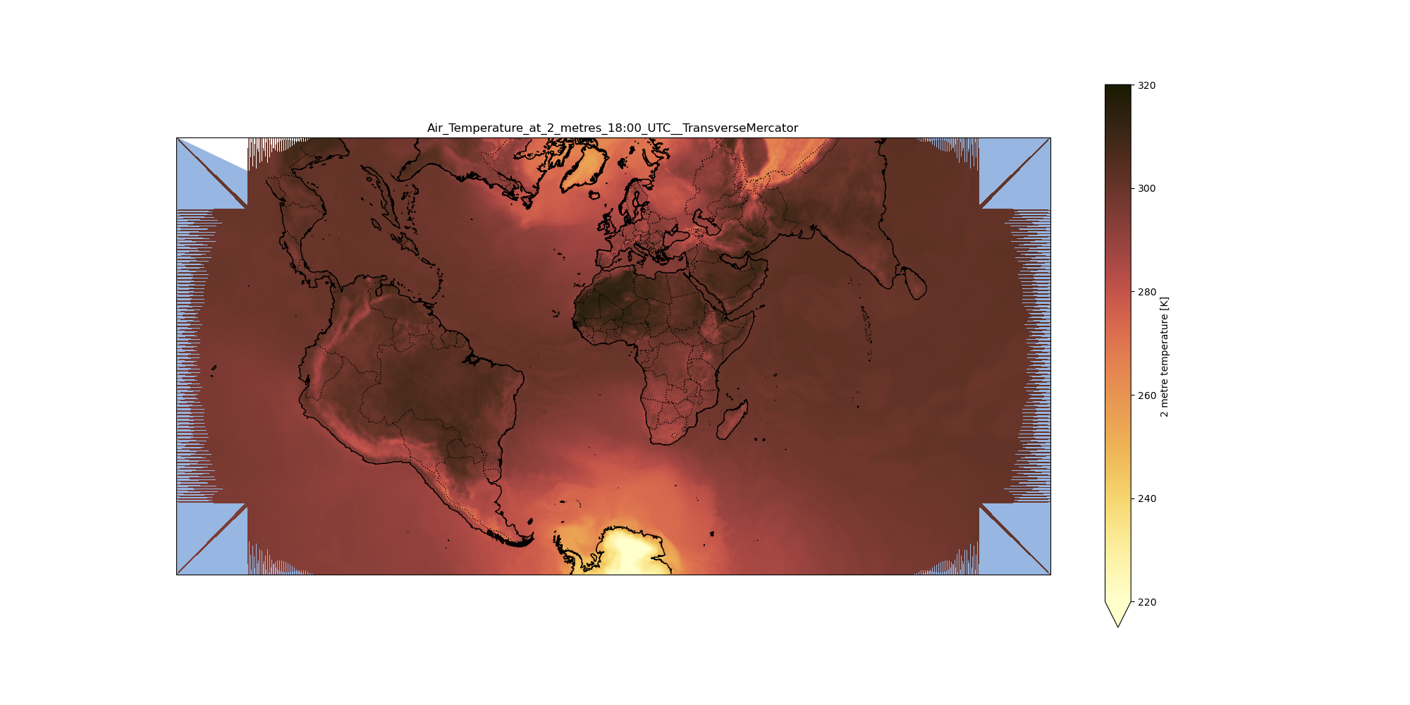
TransverseMercator Syntax:{“proj”:”TransverseMercator” }
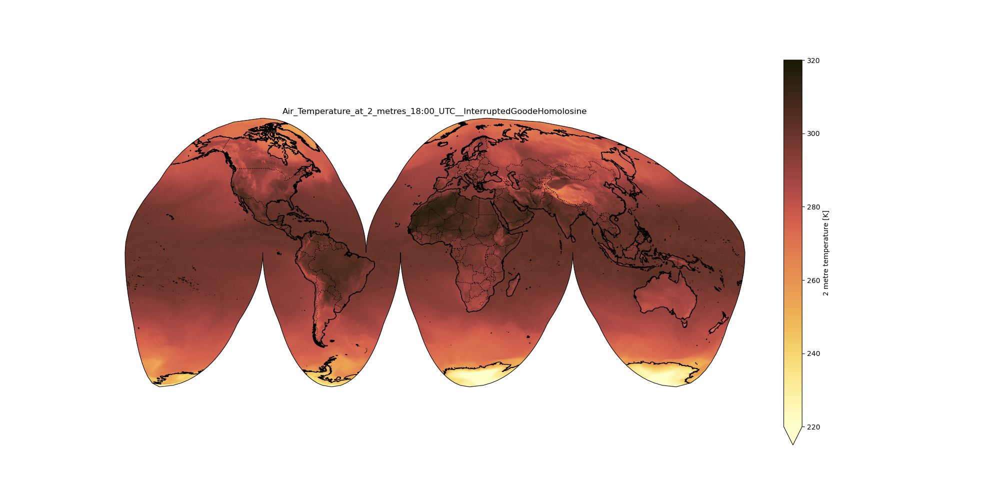
InterruptedGoodeHomolosine Syntax: {“proj”:”InterruptedGoodeHomolosine” }
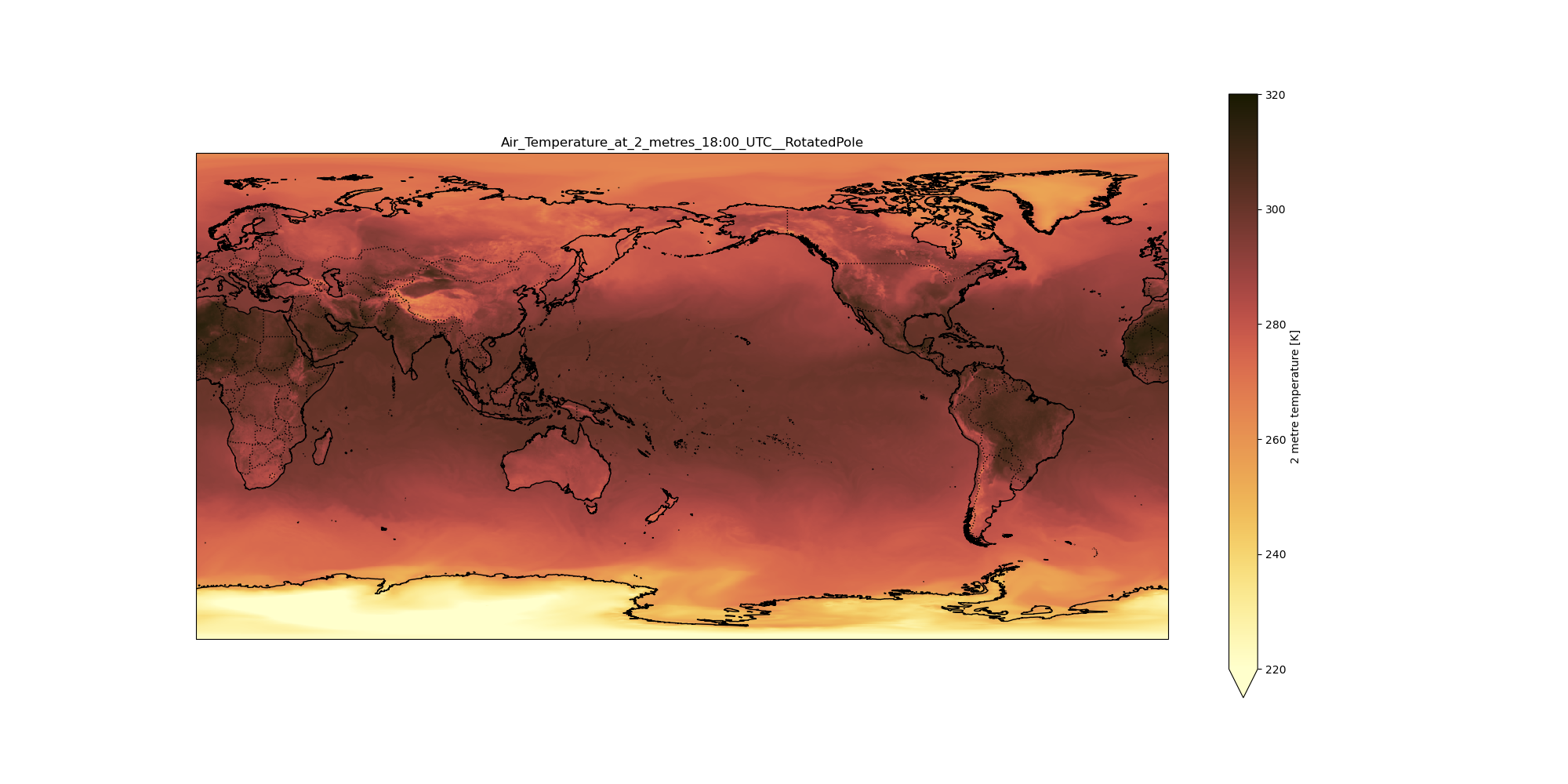
RotatedPole Syntax: {“proj”:”RotatedPole” }
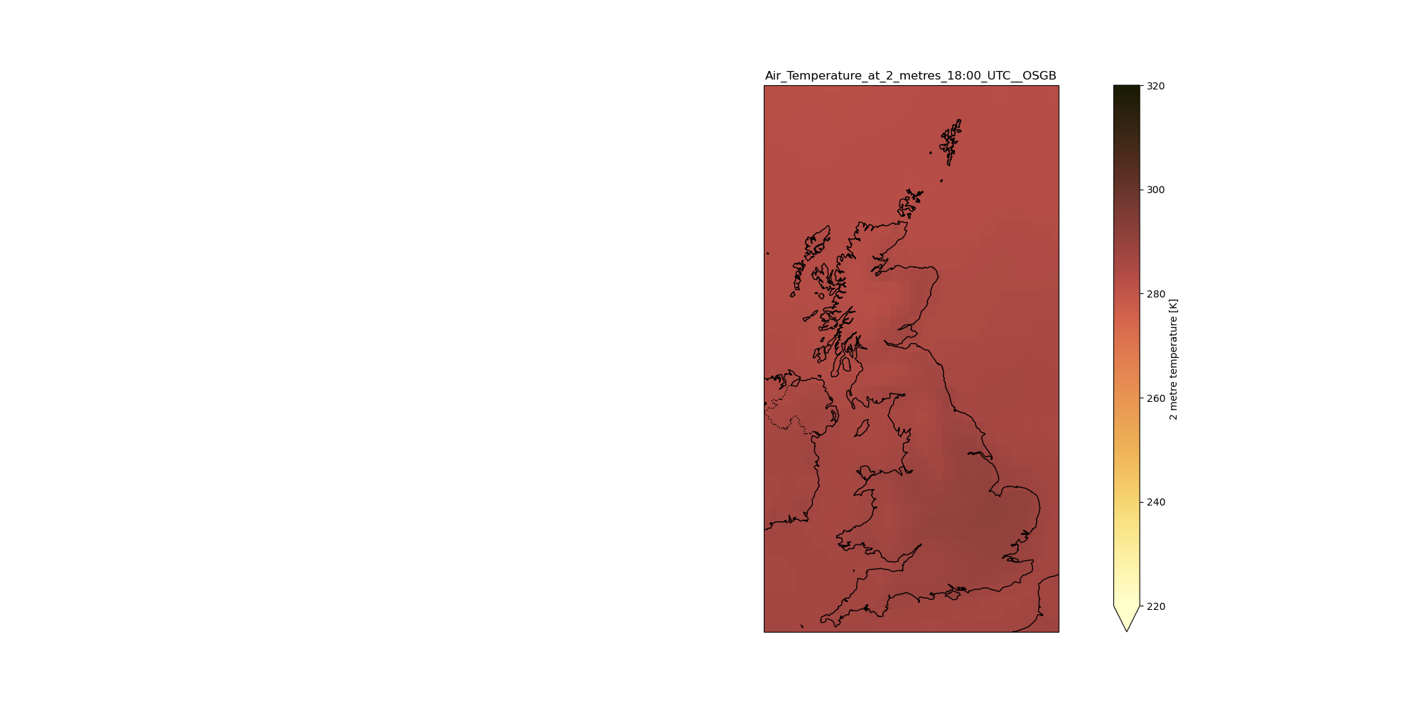
OSGB Syntax:{“proj”:”OSGB” }
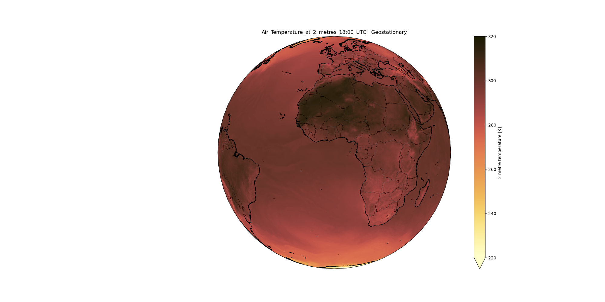
Geostationary Syntax: {“proj”:”Geostationary” }
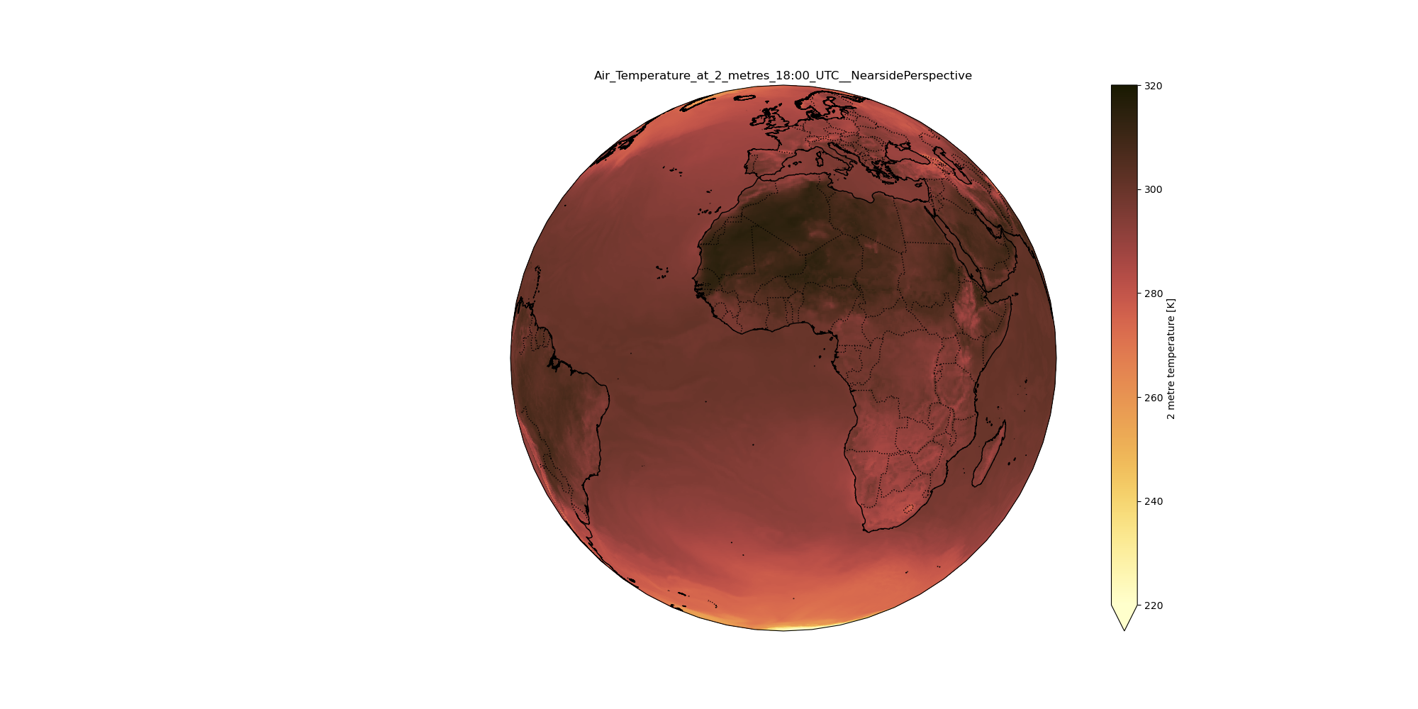
NearsidePerspective Syntax:{“proj”:”NearsidePerspective” }
EckertI Syntax: {“proj”:”EckertI” }
EckertII Syntax: {“proj”:”EckertII” }
EckertIII Syntax: {“proj”:”EckertIII” }
EckertIV Syntax: {“proj”:”EckertIV” }
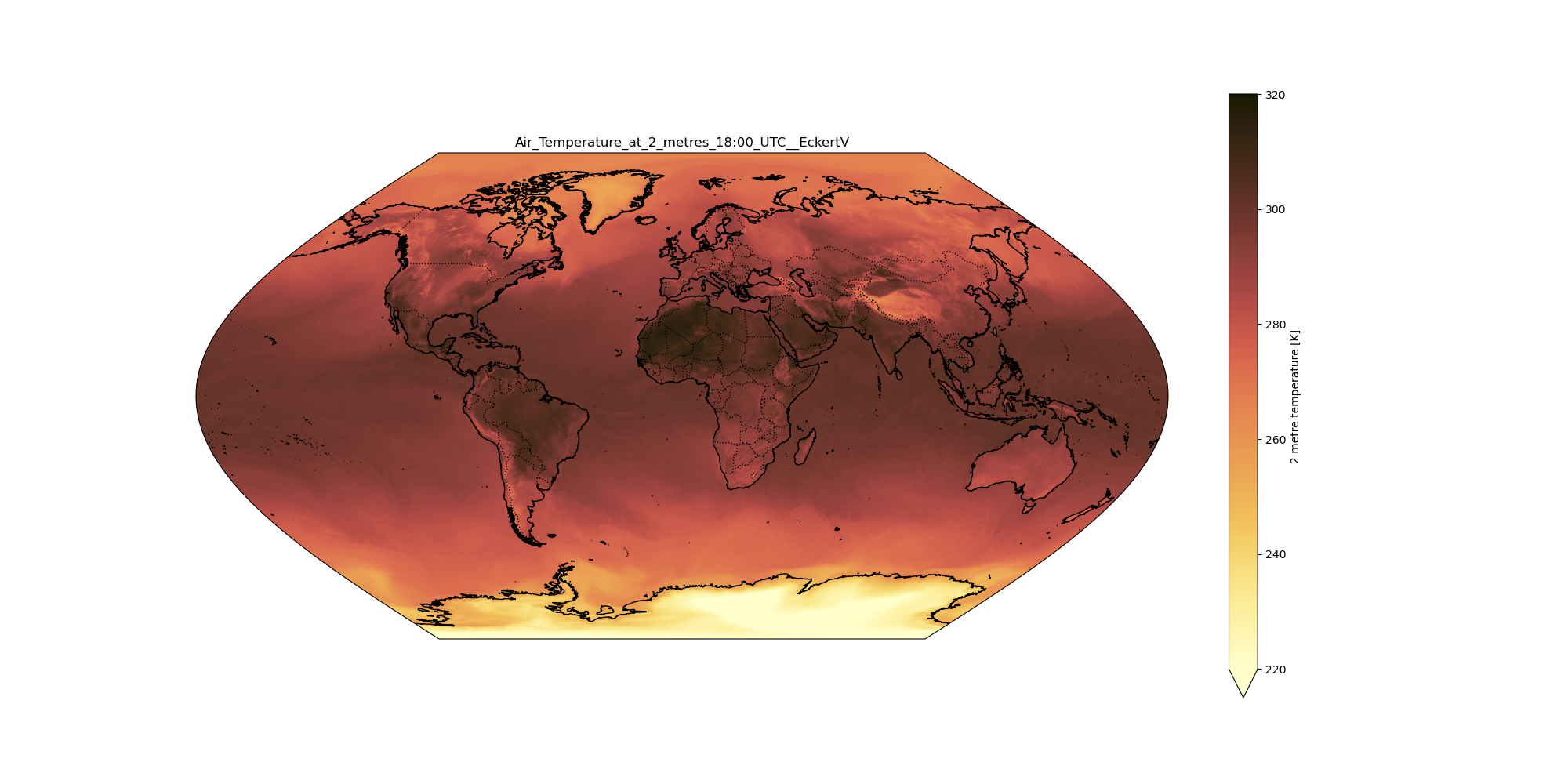
EckertV Syntax: {“proj”:”EckertV” }
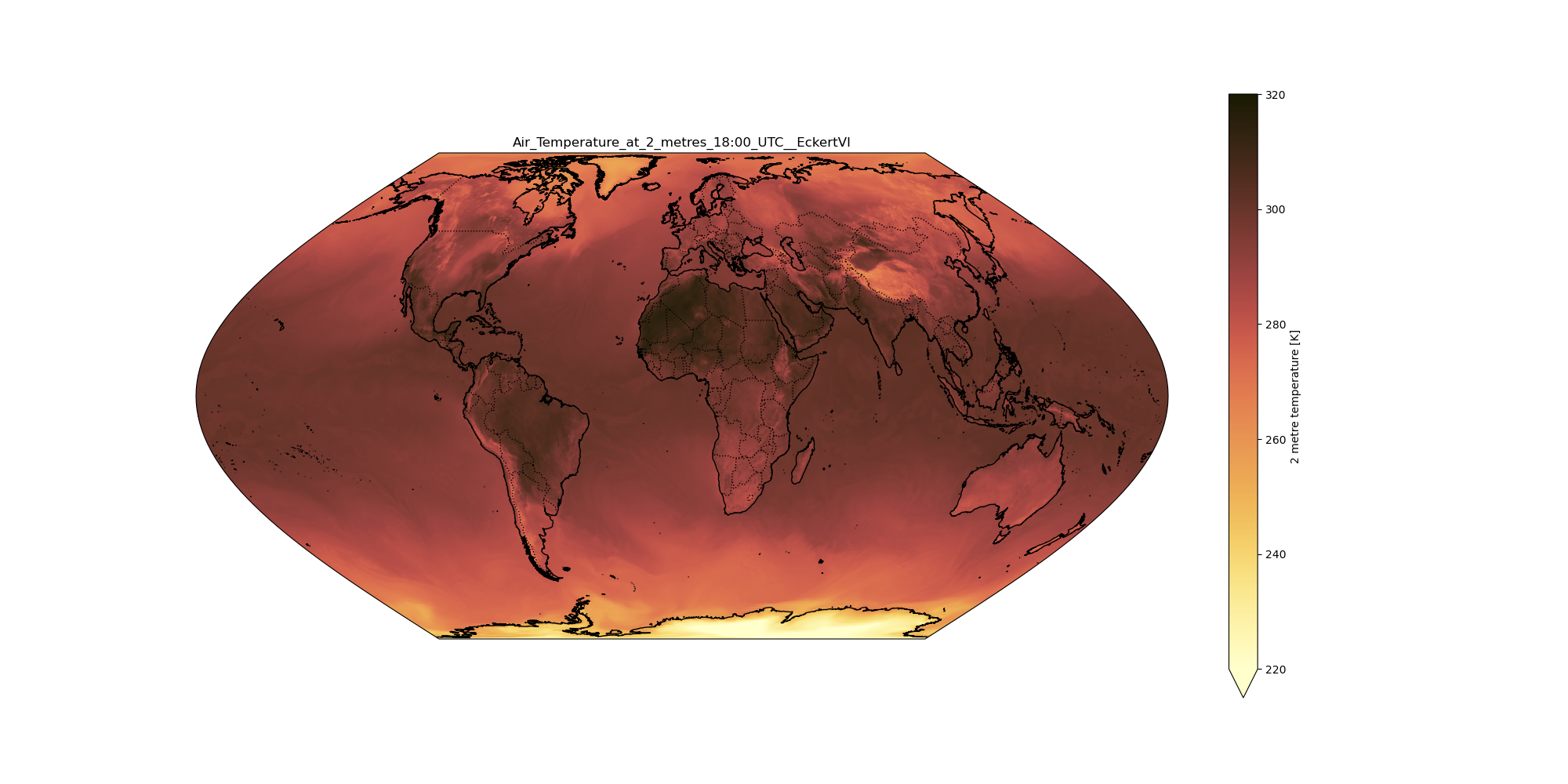
EckertVI Syntax: {“proj”:”EckertVI” }
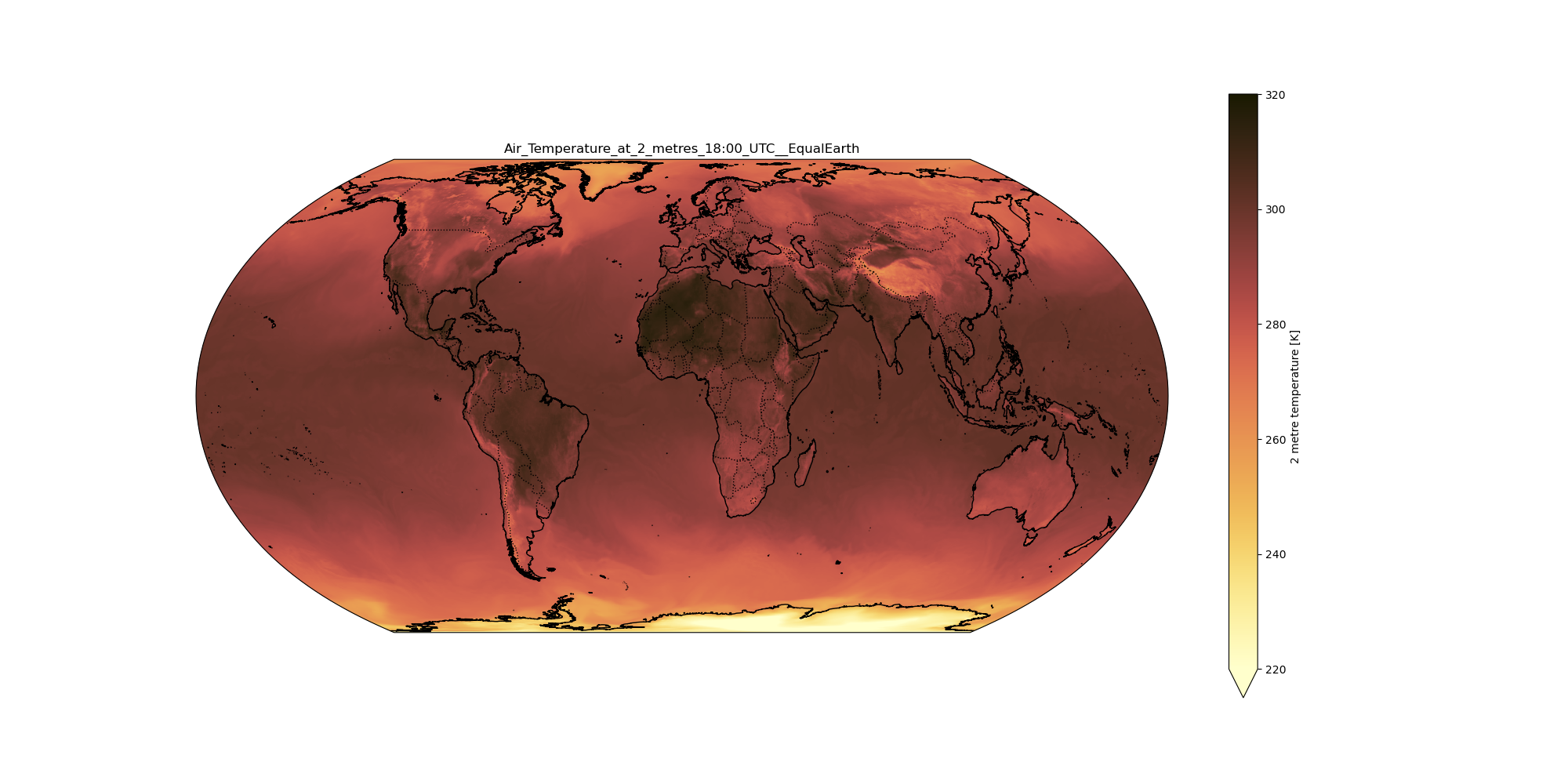
EqualEarth Syntax:{“proj”:”EqualEarth” }
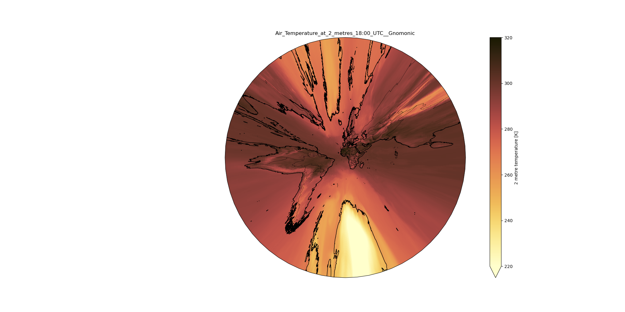
Gnomonic Syntax: {“proj”:”Gnomonic” }
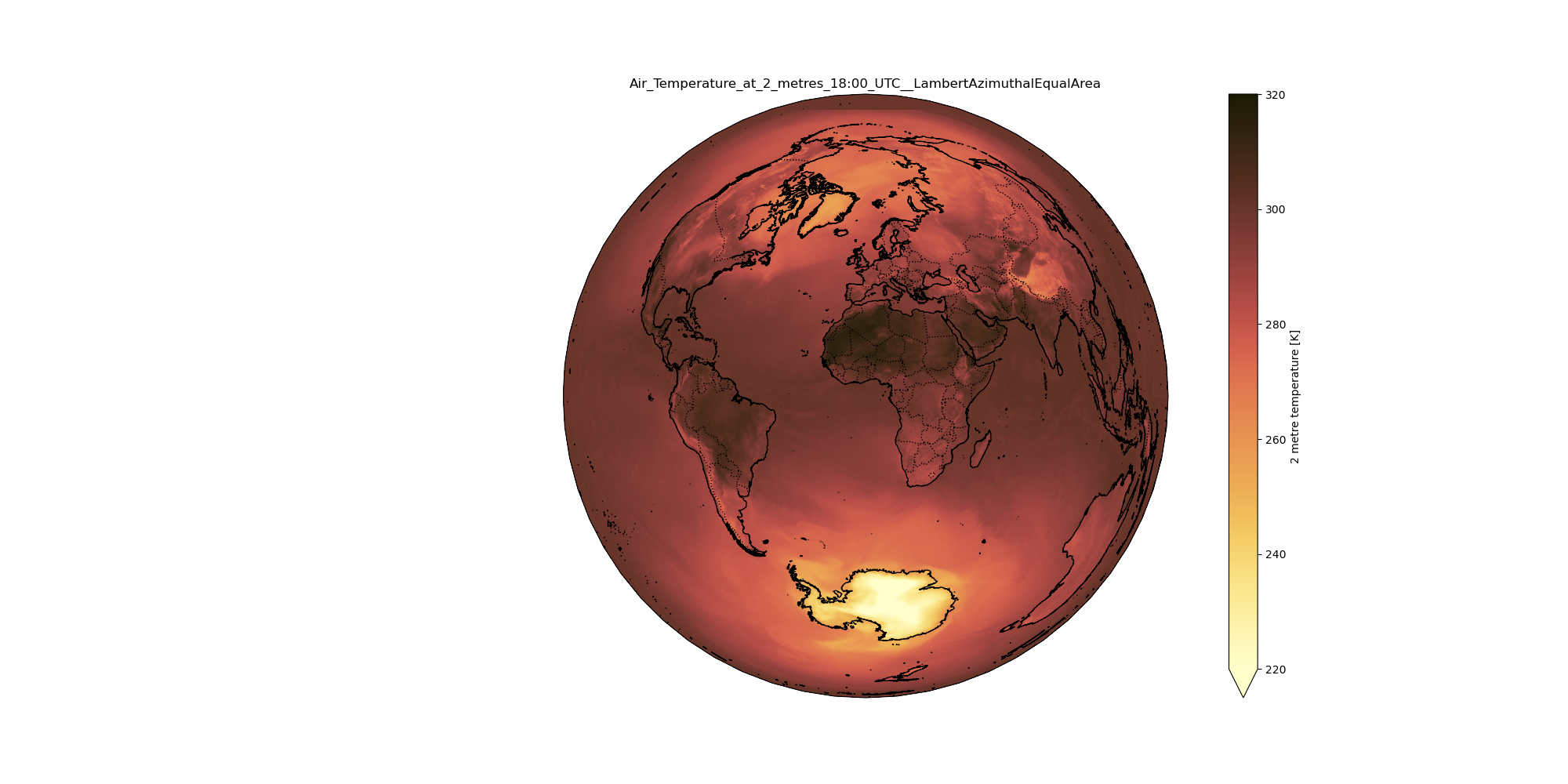
LambertAzimuthalEqualArea Syntax: {“proj”:”LambertAzimuthalEqualArea” }
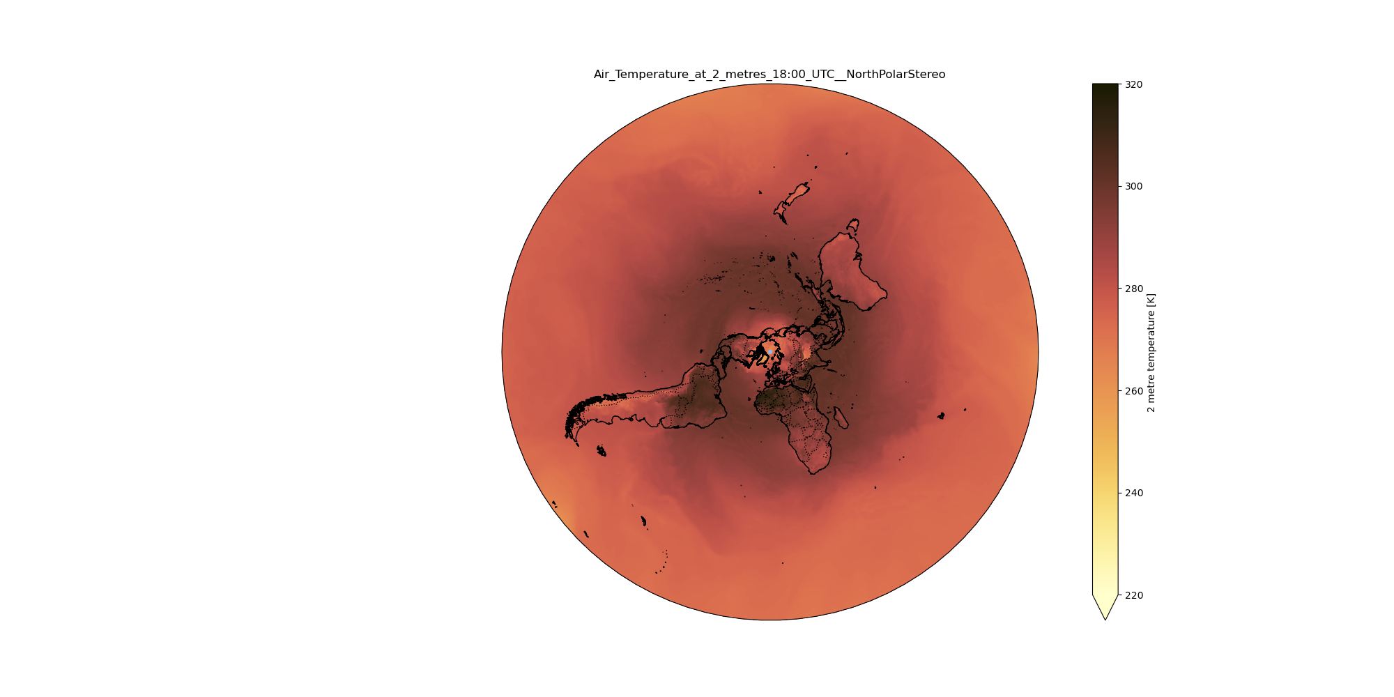
NorthPolarStereo Syntax: {“proj”:”NorthPolarStereo” }
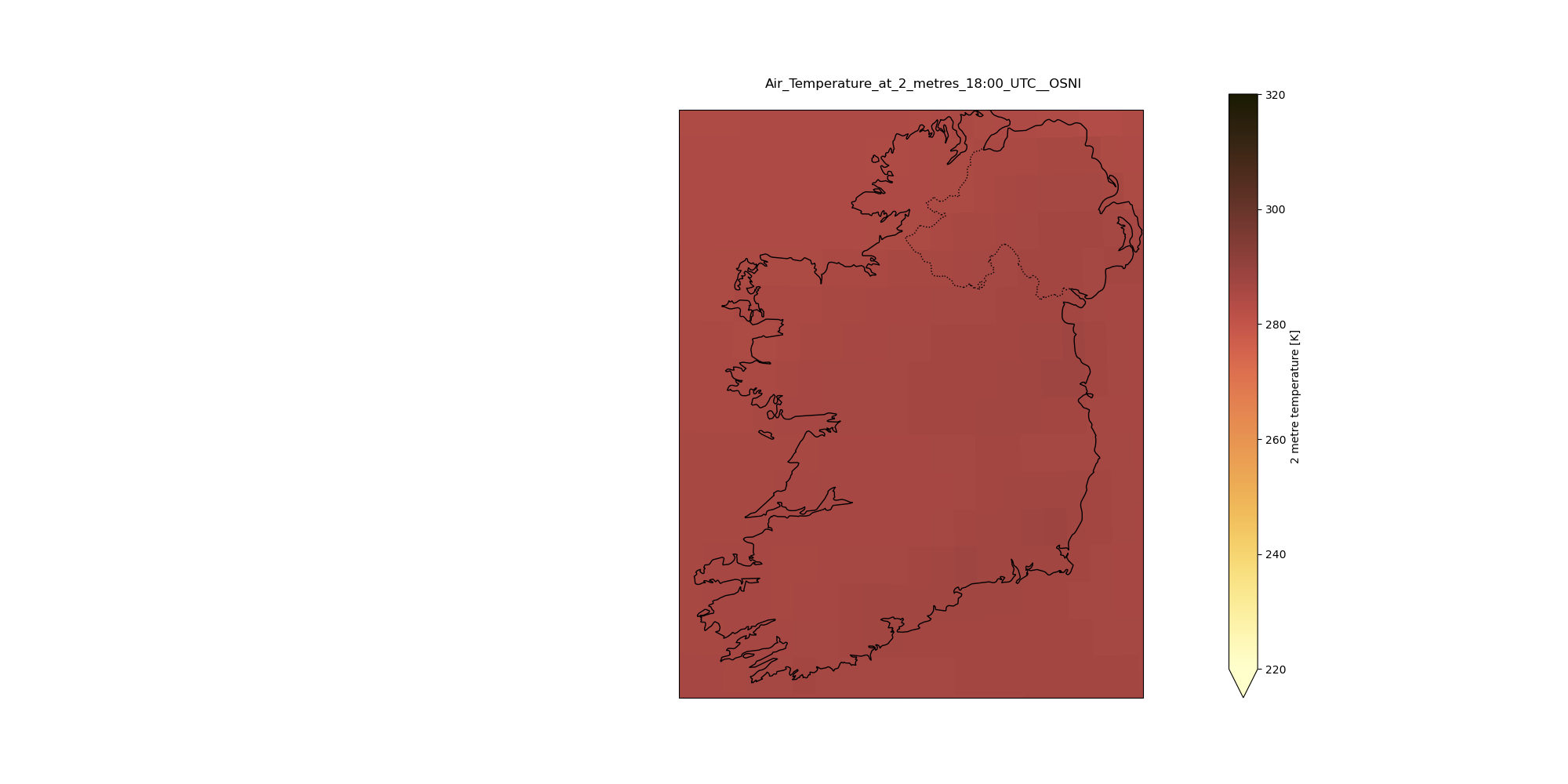
OSNI Syntax: {“proj”:”OSNI” }
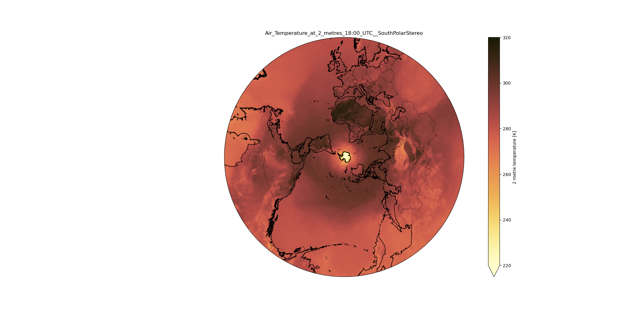
SouthPolarStereo Syntax: {“proj”:”SouthPolarStereo” }

QuestionWhat are the different kinds of projections that can be used?
There are many projections which can be used in the
NetCDF xarray map plottingtool. Different projections have different purposes and need to be carefully chosen.Plotting different projections using NetCDF xarray map plotting:
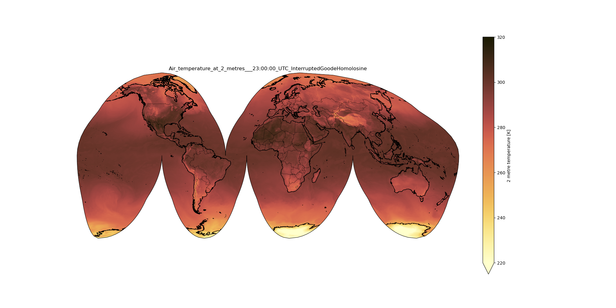
Hands On: Plotting the major projections using the xarray tool.
- NetCDF xarray map plotting ( Galaxy version 0.20.2+galaxy0) with the following parameters:
- param-file “Netcdf file”:
outfile.netcdf- param-file “Tabular of variables”:
Metadata infos from outfile.netcdf(output of NetCDF xarray Metadata Info tool)- “Choose the variable to plot”:
air_temperature_at_2_metres- “Name of latitude coordinate”:
lat- “Name of longitude coordinate”:
lon- “Datetime selection”:
No- “Range of values for plotting e.g. minimum value and maximum value (minval,maxval) (optional)”:
220,320- “Add country borders with alpha value [0-1] (optional)”:
1.0- “Add coastline with alpha value [0-1] (optional)”:
1.0- “Add ocean with alpha value [0-1] (optional)”:
1.0- “Specify plot title (optional)”:
Air_temperature_at_2_metres___23:00:00_UTC_InterruptedGoodeHomolosine- “Specify which colormap to use for plotting (optional)”:
lajolla- “Specify the projection (proj4) on which we draw e.g. {“proj”:”PlateCarree”} with double quote (optional)”:
{"proj":"InterruptedGoodeHomolosine" }The final plot is shown below:
Some other potentially interesting types of projections can be found below :
{“proj”:”LambertCylindrical” }
{“proj”:”Orthographic” }
{“proj”:”Sinusoidal” }
{“proj”:”EquidistantConic”}
{“proj”:”LambertConformal” }
{“proj”:”AzimuthalEquidistant” }

There are about 150 different kinds of maps available in the colormaps options. This document contains a list of all the types of projections and colormaps available to the users while using the Xarray Map Plotting. These depict the global air temperature at 2 metres on a Kelvin Scale of range 220 K TO 320 K. Let’s get started! Below is the complete list for reference.
ACCENT
BLUES
BrBg
BuGn
BuPu
CMRmap
Dark2
Acton
Acton_r
Afmhot
Autumn
Bam
BamO
BamO_r
Bamako
Bamako_r
Batlow
BatlowK
BatlowK_r
BatlowW
BatlowW_r
Batlow_r
Berlin
berlin_r
Bilbao
Bilbao_r
Binary
Bone
Brg
Broc
BrocO
BrocO_r
Broc_r
Buda
Buda_r
Bukavu
Bukavu_r
Bwr
Cool
Coolwarm
Copper
Cork
CorkO
CorkO_r
Cork_r
Cubehelix
Davos
GnBu
Greens
Greys
Imola
OrRd
Oranges
Paired
Pastel1
Pastel2
Davos_r
Devon_r
Devon
Fes
Fes_r
Flag
Gist_earth
Gist_gray
Gist_heat
Gist_ncar
Gist_rainbow
Gist_stern
Gist_yarg
Gnuplot
Gnuplot2
Gray
GrayC
GrayC_r
Hawaii
Hawaii_r
Hot
Hsv
Imola_r
Jet
Lajolla
Lajolla_r
Lapaz
Lapaz_r
Lisbon
Lisbon_r
Nipy_spectral
Nuuk
Nuuk_r
Ocean
Oleron
Oslo
Oslo_r
Pink
PRGn
PiYG
PuBu
PuBuGn
PuOr
PuRd
Purples
RdBu
RdBu_r
RdBu_r
RdPu
RdPu_r
RdYIBu
RdYIGn
Reds
Set1
Set2
Set3
Spectral
Wistia
YIGn
YIGnBu
YIOrBr
YIOrRd
Prism
Rainbow
Roma
RomaO
RomaO_r
Roma_r
Seismic
Spring
Summer
Tab10
Tab20
Tab20b
Tab20c
Terrain
Tofino
Tofino_r
Tokyo
Tokyo_r
Turku
Turku_r
Vanimo
Vanimo_r
Vik
VikO
VikO_r
Vik_r
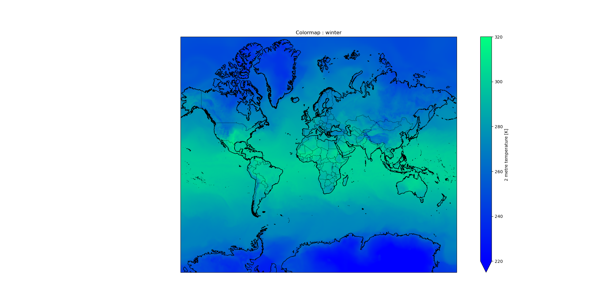
Winter
Question
- What are the different kinds of colormaps that can be used?
When it comes to conveying the correct information, through visualisation, colors play a major role. Suppose you want to display a cold region, its an obvious practice of using cooler tones such as a
blue. Thus it is important to understand the choices we have.Plotting different colormaps using NetCDF xarray map plotting
Hands On: Plotting the major colormaps using the xarray tool.
- NetCDF xarray map plotting ( Galaxy version 0.20.2+galaxy0) with the following parameters:
- param-file “Netcdf file”:
outfile.netcdf- param-file “Tabular of variables”:
Metadata infos from outfile.netcdf(output of NetCDF xarray Metadata Info tool)- “Choose the variable to plot”:
air_temperature_at_2_metres- “Name of latitude coordinate”:
lat- “Name of longitude coordinate”:
lon- “Datetime selection”:
No- “Range of values for plotting e.g. minimum value and maximum value (minval,maxval) (optional)”:
220,320- “Add country borders with alpha value [0-1] (optional)”:
1.0- “Add coastline with alpha value [0-1] (optional)”:
1.0- “Add ocean with alpha value [0-1] (optional)”:
1.0- “Specify plot title (optional)”:
Air_temperature_at_2_metres___23:00:00_UTC_batlow“Specify which colormap to use for plotting (optional)”:
batlow- “Specify the projection (proj4) on which we draw e.g. {“proj”:”PlateCarree”} with double quote (optional)”:
{'proj': 'Mercator'}The final plot is shown below:
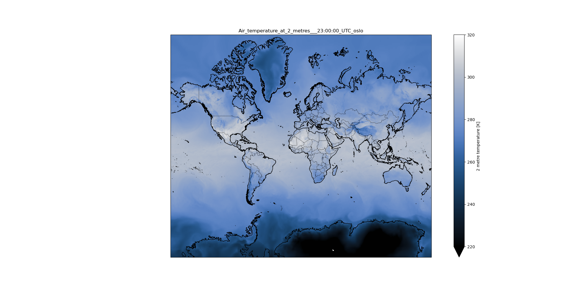
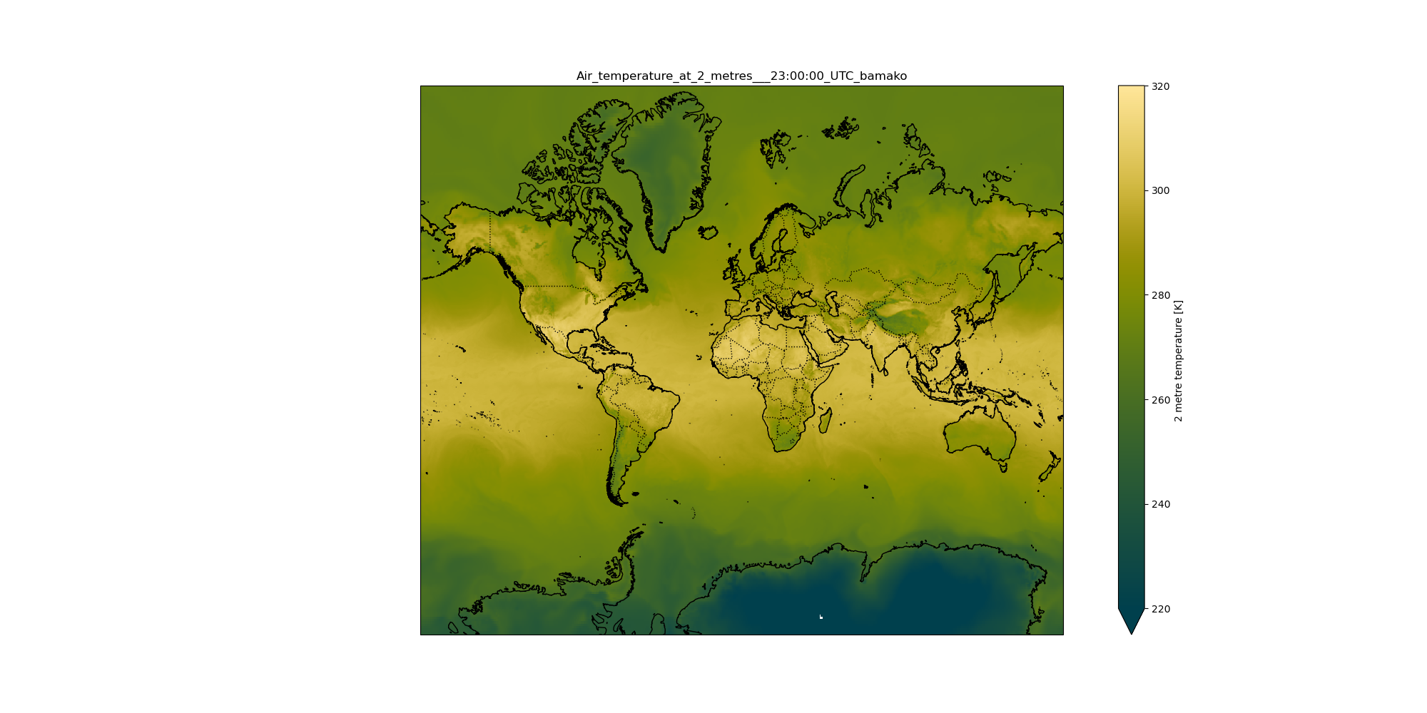
Some other important color variants of the same map can be found below :
- colormap : oslo
- colormap : bamako
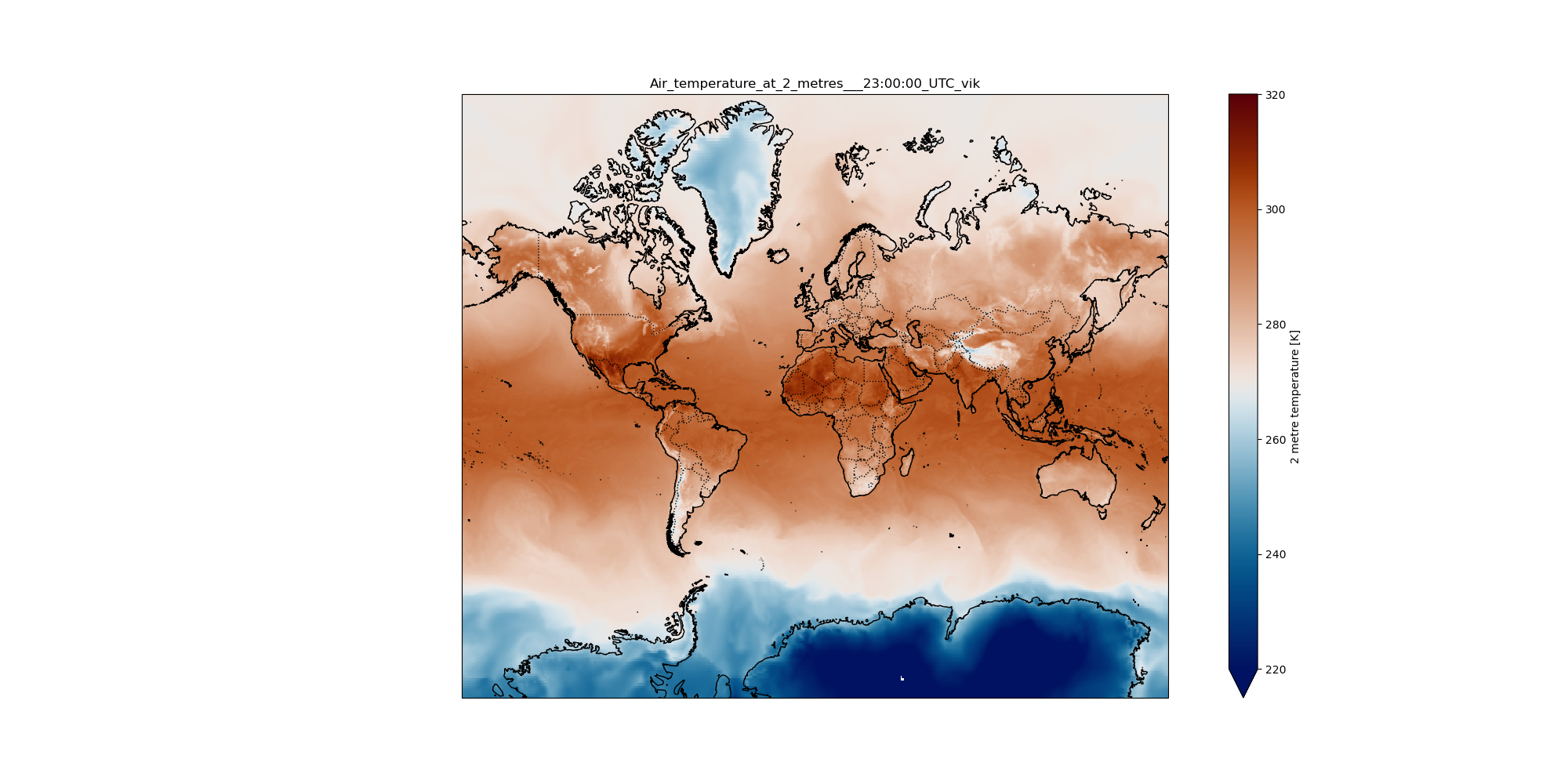
- colormap : vik
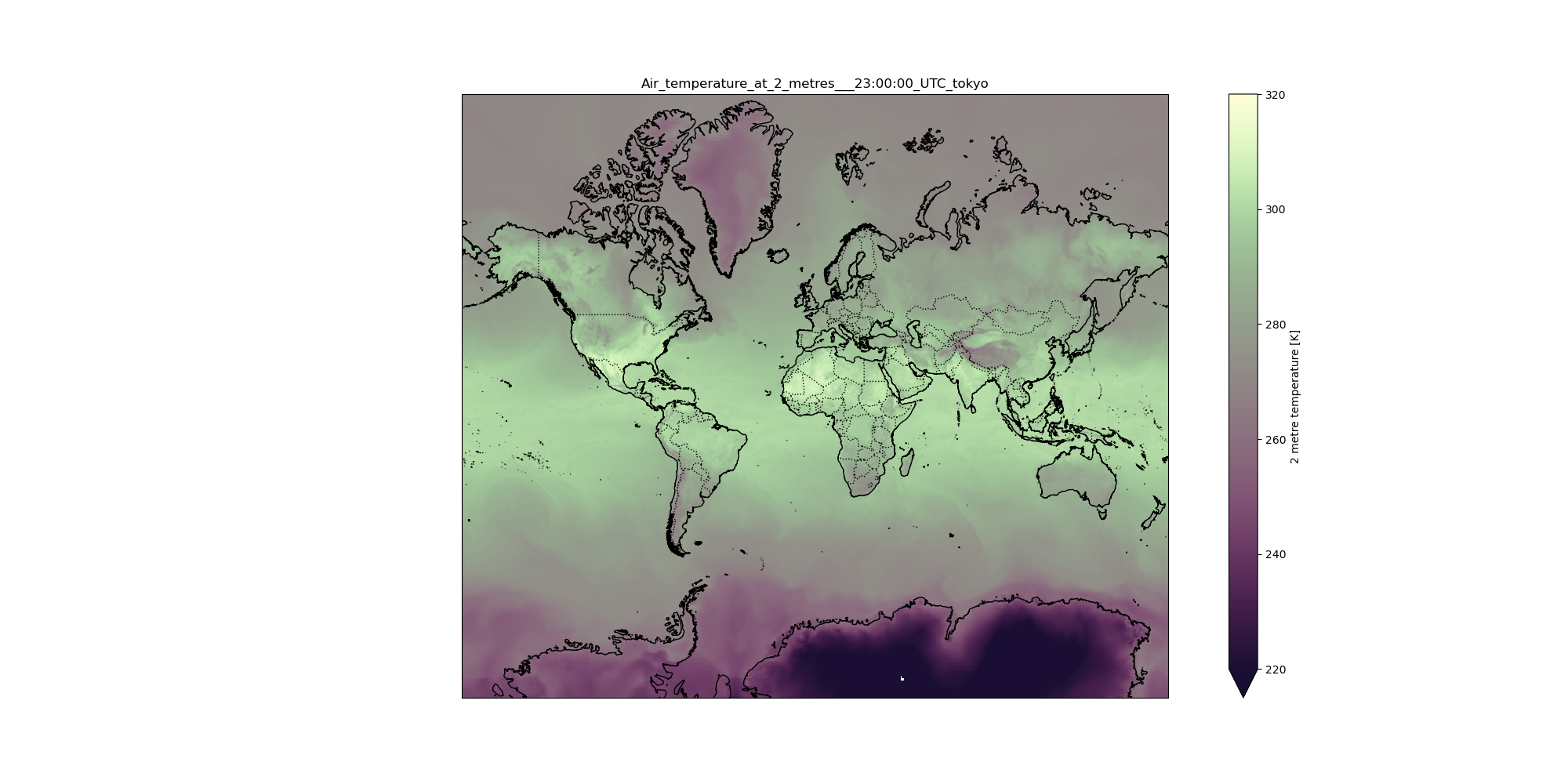
- colormap : tokyo
- colormap : hawaii
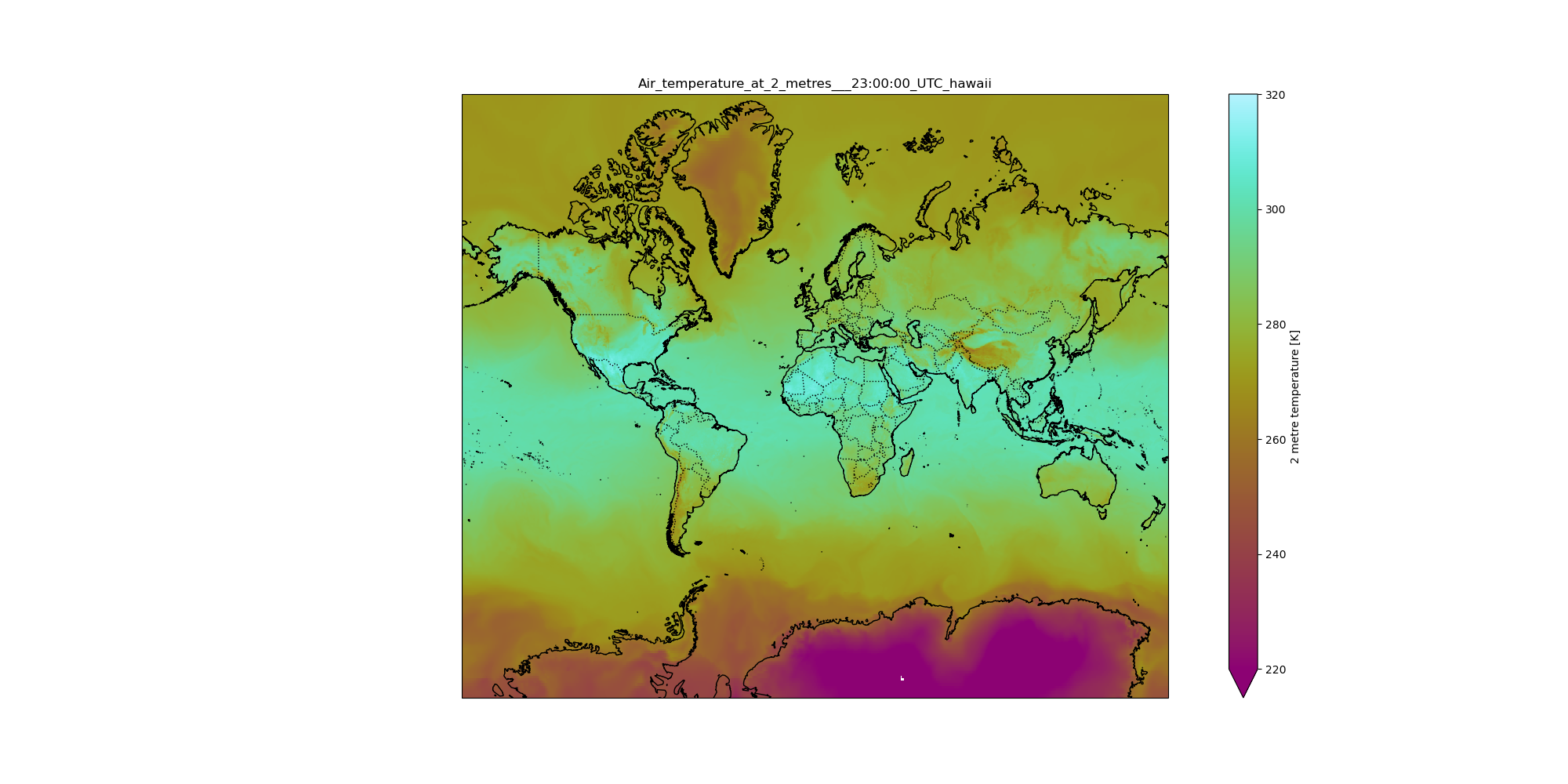
Question
- What insights can be driven from the data and how is the data important on a local level?
- What are some giveaways from the tutorial ?
- Every piece of data recites a story. The air temperature at a certain height has a lot of significance in major commercial and day to day activities. Read this data-blog on the above analysis. Click Here.
The tutorial has summed up a proper way of plotting data from a netcdf file. It has discussed everything from loading of data to its final display. Some other key points to keep in mind are :
- It may take some time while plotting the maps. It depends on traffic / load on the Galaxy server. It is suggested to have a 64-bit processor with 8GB RAM storage. Be patient.
- You can view as well as download the generated plots to use further.
- Plotting over global maps is very convinient as you saw above. But many a times, you want to plot a specific region, it becomes very easy using CDO tool. Refer to this tutorial for more info.
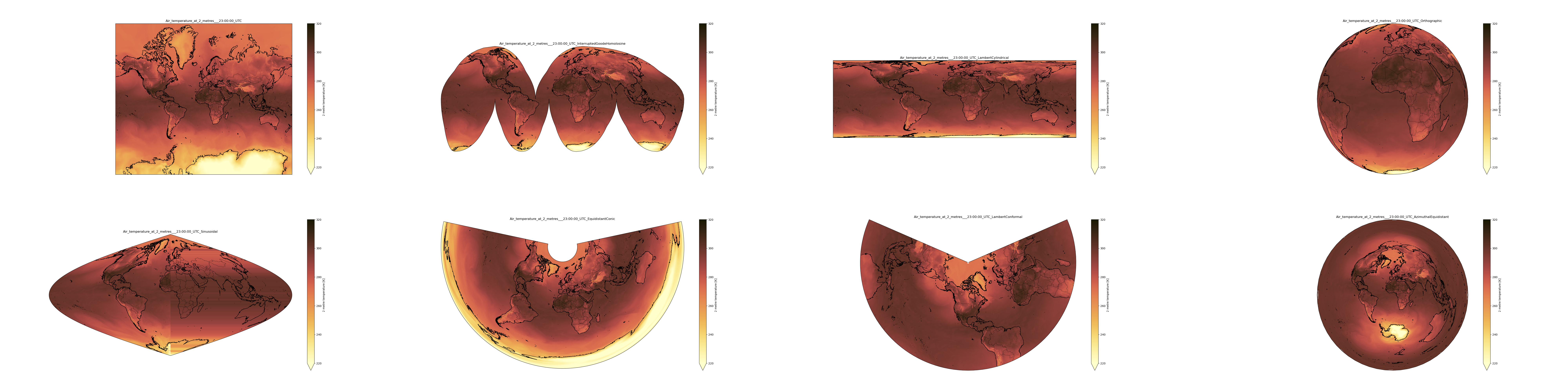
- If you wish to present all the plotted maps at one place for comparision or analysis. It is a short and simple step and can be doe using the tool name
Image Montage.Image Montage ( Galaxy version 1.3.31+galaxy1) with the following parameters:
- param-files “Images”:
Map plots- param-text ”# of images wide”:
4Here you can see that all the projections we plotted above have been shown in a single image usingImage Montage.
Conclusion
We have learnt about the xarray map plotting tool dealing with the netcdf data set. The tutorial also discussed about the types of climate datasets. One of the tutorial is info about usage of different colormaps and projections in xarray.
You've Finished the Tutorial
Key points
NetCDF xarray climate data visualization
NetCDF xarray map plotting projections
NetCDF xarray map plotting colormaps
Frequently Asked Questions
Have questions about this tutorial? Have a look at the available FAQ pages and support channelsUseful literature
Further information, including links to documentation and original publications, regarding the tools, analysis techniques and the interpretation of results described in this tutorial can be found here.
Feedback
Did you use this material as an instructor? Feel free to give us feedback on how it went.
Did you use this material as a learner or student? Click the form below to leave feedback.

Citing this Tutorial
- Soumya Jha, Visualization of Climate Data using NetCDF xarray Map Plotting (Galaxy Training Materials). https://training.galaxyproject.org/training-material/topics/ecology/tutorials/x-array-map-plot/tutorial.html Online; accessed TODAY
- Hiltemann, Saskia, Rasche, Helena et al., 2023 Galaxy Training: A Powerful Framework for Teaching! PLOS Computational Biology 10.1371/journal.pcbi.1010752
- Batut et al., 2018 Community-Driven Data Analysis Training for Biology Cell Systems 10.1016/j.cels.2018.05.012
Congratulations on successfully completing this tutorial!@misc{ecology-x-array-map-plot, author = "Soumya Jha", title = "Visualization of Climate Data using NetCDF xarray Map Plotting (Galaxy Training Materials)", year = "", month = "", day = "", url = "\url{https://training.galaxyproject.org/training-material/topics/ecology/tutorials/x-array-map-plot/tutorial.html}", note = "[Online; accessed TODAY]" } @article{Hiltemann_2023, doi = {10.1371/journal.pcbi.1010752}, url = {https://doi.org/10.1371%2Fjournal.pcbi.1010752}, year = 2023, month = {jan}, publisher = {Public Library of Science ({PLoS})}, volume = {19}, number = {1}, pages = {e1010752}, author = {Saskia Hiltemann and Helena Rasche and Simon Gladman and Hans-Rudolf Hotz and Delphine Larivi{\`{e}}re and Daniel Blankenberg and Pratik D. Jagtap and Thomas Wollmann and Anthony Bretaudeau and Nadia Gou{\'{e}} and Timothy J. Griffin and Coline Royaux and Yvan Le Bras and Subina Mehta and Anna Syme and Frederik Coppens and Bert Droesbeke and Nicola Soranzo and Wendi Bacon and Fotis Psomopoulos and Crist{\'{o}}bal Gallardo-Alba and John Davis and Melanie Christine Föll and Matthias Fahrner and Maria A. Doyle and Beatriz Serrano-Solano and Anne Claire Fouilloux and Peter van Heusden and Wolfgang Maier and Dave Clements and Florian Heyl and Björn Grüning and B{\'{e}}r{\'{e}}nice Batut and}, editor = {Francis Ouellette}, title = {Galaxy Training: A powerful framework for teaching!}, journal = {PLoS Comput Biol} }
You can use Ephemeris's
shed-tools installcommand to install the tools used in this tutorial.shed-tools install [-g GALAXY] [-a API_KEY] -t <(curl https://training.galaxyproject.org/training-material/api/topics/ecology/tutorials/x-array-map-plot/tutorial.json | jq .admin_install_yaml -r)Alternatively you can copy and paste the following YAML
---
install_tool_dependencies: true
install_repository_dependencies: true
install_resolver_dependencies: true
tools:
- name: graphicsmagick_image_montage
  owner: bgruening
  revisions: a0f01c777820
  tool_panel_section_label: Convert Formats
  tool_shed_url: https://toolshed.g2.bx.psu.edu/
- name: cdo_operations
  owner: climate
  revisions: d5355f6fa02b
  tool_panel_section_label: Climate Analysis
  tool_shed_url: https://toolshed.g2.bx.psu.edu/
- name: xarray_coords_info
  owner: ecology
  revisions: 3e73f657a998
  tool_panel_section_label: GIS Data Handling
  tool_shed_url: https://toolshed.g2.bx.psu.edu/
- name: xarray_mapplot
  owner: ecology
  revisions: dc05bf0af58f
  tool_panel_section_label: GIS Data Handling
  tool_shed_url: https://toolshed.g2.bx.psu.edu/
- name: xarray_metadata_info
  owner: ecology
  revisions: e8650cdf092f
  tool_panel_section_label: GIS Data Handling
  tool_shed_url: https://toolshed.g2.bx.psu.edu/