Sometimes there is quite a long list of genes to interpret after a differential expression analysis, and it is usually infeasible to go through the list one gene at a time trying to understand it’s biological function. A common downstream procedure is gene set testing, which aims to understand which pathways/gene networks the differentially expressed genes are implicated in. There are many different gene set testing methods that can be applied and it can be useful to try several.
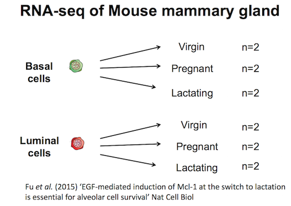
The purpose of this tutorial is to demonstrate how to perform gene set testing using tools in Galaxy. The data comes from a Nature Cell Biology paper, EGF-mediated induction of Mcl-1 at the switch to lactation is essential for alveolar cell survival), Fu et al. 2015. That study examined the expression profiles of basal and luminal cells in the mammary gland of virgin, pregnant and lactating mice (see Figure below). How to generate differentially expressed genes from reads (FASTQs) for this dataset is covered in the accompanying tutorials RNA-seq reads to counts and RNA-seq counts to genes. This tutorial is inspired by material from the COMBINE R RNAseq workshop here and the Cancer Research UK workshop here.
Your results may be slightly different from the ones presented in this tutorial due to differing versions of tools, reference data, external databases, or because of stochastic processes in the algorithms.
We will use several files for this analysis:
Differentially expressed results files (genes in rows, logFC and P values in columns)
Sample information file (sample id, group)
Gene lengths file (genes, lengths)
Filtered counts file (genes in rows, counts for samples in columns, with lowly expressed genes removed)
Gene sets file for MSigDB Hallmark collection for mouse (rdata)
Import data
Hands On: Data upload
Create a new history for this RNA-seq exercise e.g. RNA-seq genes to pathways
To create a new history simply click the new-history icon at the top of the history panel:
Click on galaxy-pencil (Edit) next to the history name (which by default is “Unnamed history”)
Type the new name
Click on Save
To cancel renaming, click the galaxy-undo “Cancel” button
If you do not have the galaxy-pencil (Edit) next to the history name (which can be the case if you are using an older version of Galaxy) do the following:
Click on Unnamed history (or the current name of the history) (Click to rename history) at the top of your history panel
Type the new name
Press Enter
Import the files, there are two options:
Option 1: From a shared data library if available (ask your instructor)
As an alternative to uploading the data from a URL or your computer, the files may also have been made available from a shared data library:
Go into Libraries (left panel)
Navigate to the correct folder as indicated by your instructor.
On most Galaxies tutorial data will be provided in a folder named GTN - Material –> Topic Name -> Tutorial Name.
Select the desired files
Click on Add to Historygalaxy-dropdown near the top and select as Datasets from the dropdown menu
In the pop-up window, choose
“Select history”: the history you want to import the data to (or create a new one)
Add a tag called #basal to the limma-voom_basalpregnant-basallactate and a tag called #luminal to the limma-voom_luminalpregnant-luminallactate files.
Datasets can be tagged. This simplifies the tracking of datasets across the Galaxy interface. Tags can contain any combination of letters or numbers but cannot contain spaces.
To tag a dataset:
Click on the dataset to expand it
Click on Add Tagsgalaxy-tags
Add tag text. Tags starting with # will be automatically propagated to the outputs of tools using this dataset (see below).
Press Enter
Check that the tag appears below the dataset name
Tags beginning with # are special!
They are called Name tags. The unique feature of these tags is that they propagate: if a dataset is labelled with a name tag, all derivatives (children) of this dataset will automatically inherit this tag (see below). The figure below explains why this is so useful. Consider the following analysis (numbers in parenthesis correspond to dataset numbers in the figure below):
a set of forward and reverse reads (datasets 1 and 2) is mapped against a reference using Bowtie2 generating dataset 3;
dataset 3 is used to calculate read coverage using BedTools Genome Coverageseparately for + and - strands. This generates two datasets (4 and 5 for plus and minus, respectively);
datasets 4 and 5 are used as inputs to Macs2 broadCall datasets generating datasets 6 and 8;
datasets 6 and 8 are intersected with coordinates of genes (dataset 9) using BedTools Intersect generating datasets 10 and 11.
Now consider that this analysis is done without name tags. This is shown on the left side of the figure. It is hard to trace which datasets contain “plus” data versus “minus” data. For example, does dataset 10 contain “plus” data or “minus” data? Probably “minus” but are you sure? In the case of a small history like the one shown here, it is possible to trace this manually but as the size of a history grows it will become very challenging.
The right side of the figure shows exactly the same analysis, but using name tags. When the analysis was conducted datasets 4 and 5 were tagged with #plus and #minus, respectively. When they were used as inputs to Macs2 resulting datasets 6 and 8 automatically inherited them and so on… As a result it is straightforward to trace both branches (plus and minus) of this analysis.
We would like to know if there are biological categories that are enriched among the differentially expressed genes. To do this we will perform a Gene Ontology analysis, similar to the RNA-seq ref-based tutorial.
Gene Ontology (GO) analysis is widely used to reduce complexity and highlight biological processes in genome-wide expression studies. However, standard methods give biased results on RNA-seq data due to over-detection of differential expression for long and highly-expressed transcripts.
The goseq tool provides methods for performing GO analysis of RNA-seq data, taking length bias into account. The methods and software used by goseq are equally applicable to other category based tests of RNA-seq data, such as KEGG pathway analysis.
goseq needs 2 files as inputs:
a differentially expressed genes file. Information for all genes tested for differential expression (all genes after filtering lowly expressed). This file should have 2 columns:
the Gene IDs (unique within the file)
True (differentially expressed) or False (not differentially expressed)
a gene lengths file. Information to correct for potential length bias in differentially expressed genes. This file should have 2 columns:
the Gene IDs (unique within the file)
the gene lengths
We need a table of differentially expressed (DE) results for goseq. Here we will use two tables, one for each of the basal and luminal pregnant vs lactate results. This is so we can compare results for the two cell types. These tables were output from the limma-voom tool but DE tables from edgeR or DESeq2 could also be used. For this dataset we will call genes differentially expressed if they have an adjusted P value below 0.01. We can use the gene lengths from the counts table in GEO (provided as a file called seqdata in Zenodo). But if we didn’t have that we could use a tool like featureCountstool to output a gene lengths file. The seqdata file contains >20k genes, but we only want the ~15k we have in our differentially expressed genes file. So we will join the lengths file with the differentially expressed genes file, keeping only the length information for genes present in the differentially expressed genes file. We can then cut out the columns we need for the two inputs (gene id, length) (gene id, DE status) and as a bonus they will both be sorted in the same order, which is what we need for goseq.
To generate the two input files we will use:
Compute to add a column to the DE tables, that gives genes meeting our adj.P threshold the value “True” and all other genes the value “False”.
Join two Datasets to add the gene length information to the differentially expressed genes, matching on gene ids
Cut to extract the two columns for the differentially expressed genes information
Cut to extract the two columns for the gene length information
Hands On: Prepare the two inputs for GOSeq
Compute an expression on every rowtool with the following parameters:
param-file“as a new column to”: the limma-voom_basalpregnant-basallactate file
param-select“Skip a header line”: yes
param-select“The new column name”: Status
Join two Datasets side by side on a specified fieldtool with the following parameters:
param-file“Join”: output of Computetool
param-select“using column”: Column: 1
param-file“with” the seqdata file
param-select“and column”: Column: 1
param-select“Keep the header lines”: Yes
Cut columns from a tabletool with the following parameters:
param-text“Cut columns”: c1,c10 (the gene ids and DE status)
param-select“Delimited by”: Tab
param-file“From”: output of Jointool
Rename to goseq DE status
Cut columns from a tabletool with the following parameters:
param-text“Cut columns”: c1,c12 (the gene ids and lengths)
param-select“Delimited by”: Tab
param-file“From”: output of Jointool
Rename to goseq gene lengths
We now have the two required input files for goseq.
Hands On: Perform GO analysis
goseqtool with
param-file“Differentially expressed genes file”: goseq DE status
param-file“Gene lengths file”: goseq gene lengths
param-select“Gene categories”: Get categories
param-select“Select a genome to use”: Mouse(mm10)
param-select“Select Gene ID format”: Entrez Gene ID
param-check“Select one or more categories”: GO: Biological Process
“Output Options”
param-check“Output Top GO terms plot?”Yes
goseq generates a big table with the following columns for each GO term:
category: GO category
over_rep_pval: p-value for over representation of the term in the differentially expressed genes
under_rep_pval: p-value for under representation of the term in the differentially expressed genes
numDEInCat: number of differentially expressed genes in this category
numInCat: number of genes in this category
term: detail of the term
ontology: MF (Molecular Function - molecular activities of gene products), CC (Cellular Component - where gene products are active), BP (Biological Process - pathways and larger processes made up of the activities of multiple gene products)
p.adjust.over_represented: p-value for over representation of the term in the differentially expressed genes, adjusted for multiple testing with the Benjamini-Hochberg procedure
p.adjust.under_represented: p-value for over representation of the term in the differentially expressed genes, adjusted for multiple testing with the Benjamini-Hochberg procedure
To identify categories significantly enriched/unenriched below some p-value cutoff, it is necessary to use the adjusted p-value.
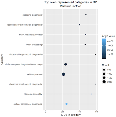
A plot of the top 10 over-represented GO terms (by p-value) can be output from the goseq tool to help visualise results. Click on the Top over-represented GO terms plot PDF in the history. It should look similar to below.
Figure 2: Basal pregnant vs lactating top 10 GO terms
Question
Can you generate the plot of top 10 GO terms for the luminal differentially expressed genes? Tip: You could use the Rerun button for each step (as the parameters are already selected) and choose the luminal file as input.
Running goseq on the luminal file should give a plot similar to below.
Figure 3: Luminal pregnant vs lactating top 10 GO terms
For more on GO analysis, including how to simplify GO results and visualize with GO graphs, see the GO Enrichment tutorial.
Gene Set Enrichment Analysis with fgsea
Gene Set Enrichment Analysis (GSEA) (Subramanian et al., 2005) is a widely used method that determines whether a set of genes is enriched in a list of differentially expressed genes. Unlike the previous method with goseq, no threshold is applied for what is considered “differentially expressed”, all genes are used. If a gene set falls at either the top (over-expressed) or bottom (under-expressed) of the list it is said to be enriched. fgsea is a faster implementation of the GSEA method. fgsea requires a ranked list of genes and some gene sets to test.
The Molecular Signatures Database (MSigDB) contains curated collections of gene sets that are commonly used in a GSEA analysis. They can be downloaded from the Broad website. But these collections are only of human gene sets. If working with another species you would need to first map the genes to their human orthologues. However, MSigDB versions for mouse are provided by the Smyth lab here. There are several MSigDB collections, we’ll use the Hallmark collection, which contains 50 gene sets. According to MSigDB, “each gene set in the hallmark collection consists of a “refined” gene set, derived from multiple “founder” sets, that conveys a specific biological state or process and displays coherent expression. The hallmarks effectively summarize most of the relevant information of the original founder sets and, by reducing both variation and redundancy, provide more refined and concise inputs for gene set enrichment analysis”. We’ll use the mouse Hallmark file provided in Zenodo, originally downloaded from http://bioinf.wehi.edu.au/software/MSigDB/mouse_H_v5p2.rdata.
There are several ways we could choose to rank our genes, we could rank by log-fold change (most upregulated to most downregulated) but that doesn’t take into account any error in the log fold change value. Another way is to use the “signed fold change” which is to rank by the sign of the fold change multiplied by the P value (as described here. We could also use the t statistic that’s output from limma, as that takes into account the log-fold change and it’s standard error, see here for more explanation. We’ll use the t statistic to rank here.
Hands On: Perform gene set enrichment with fgsea
Cut columns from a tabletool with
param-text“Cut columns”: c1,c6 (the Entrez gene ids and t-statistic)
param-select“Delimited by”: Tab
param-file“From”: the limma-voom_basalpregnant-basallactate file
Sort data in ascending or descending ordertool with
param-file“Sort Query”: the output of Cuttool
param-text“Number of header lines”: 1
“Column selections”:
param-select“on column”: Column: 2
param-select“in”: Descending order
param-select“Flavor”: Fast numeric sort (-n)
fgseatool with
param-file“Ranked Genes”: the output of Sorttool
param-check“File has header?”: Yes
param-file“Gene Sets”: mouse_hallmark_sets (this should be rdata format, if not, see how to change it in the Tip below)
param-text“Minimum Size of Gene Set”: 15
param-check“Output plots”: Yes
Click on the galaxy-pencilpencil icon for the dataset to edit its attributes
In the central panel, click galaxy-chart-select-dataDatatypes tab on the top
In the galaxy-chart-select-dataAssign Datatype, select your desired datatype from “New Type” dropdown
Tip: you can start typing the datatype into the field to filter the dropdown menu
Click the Save button
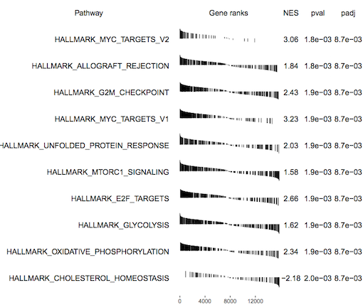
fgsea outputs a table of results containing a list of pathways with P values and enrichment scores. It can also output a summary table plot of the top pathways such as the one shown below for the basallpregnant-basallactate contrast below.
An enrichment plot of the each of the top pathways can also be produced, one is shown below. The barcode pattern shows where the genes in the set are found in the list of ranked genes. Most of the bars to the left indicate enrichment of the set at the top of the ranked list of genes (upregulated) and most bars towards the right indicate enrichment at the bottom of the list (downregulated). The enrichment score reflects the degree to which the genes are enriched at the top or bottom of the list.
The ensemble of genes set enrichment analyses (EGSEA) (Alhamdoosh et al, 2017) is a method developed for RNA-seq data that combines results from multiple algorithms and calculates collective gene set scores, to try to improve the biological relevance of the highest ranked gene sets. EGSEA has built-in gene sets from MSigDB and KEGG for human and mouse. We’ll show here how it can be used with the MSigDB Hallmark collection and KEGG pathways. For input we need a count matrix and EGSEA will perform a limma-voom analysis before gene set testing. We can use the provided filtered counts file output from limma, where the low count genes have been filtered out (output from limma by selecting “Output Filtered Counts Table?”: Yes). We just need to remove the gene symbol and description columns. We also need a symbols mapping file containing just the Entrez ids and symbols, which we can generate from the filtered counts file. The third input we need is a factors information file, containing what groups the samples belong to, we can use the same one from the tutorial RNA-seq counts to genes. EGSEA provides twelve base methods and we will select eleven, all except roast, as the fry method is a fast approximation of roast.
Hands On: Perform ensemble gene set testing with EGSEA
Cut columns from a table (cut)tool with the following parameters:
param-file“File to cut”: limma-voom filtered counts
param-select“Operation”: Discard
param-select“List of fields”: Select Column:2, Column:3
Rename to EGSEA counts
Cut columns from a table (cut)tool with the following parameters:
param-file“File to cut”: limma-voom filtered counts
param-select“Operation”: Keep
param-select“List of fields”: Select Column:1, Column:2
Rename to EGSEA anno
EGSEAtool with the following parameters:
param-select“Count Files or Matrix?”: Single Count Matrix
param-file“Count Matrix”: Select EGSEA counts
param-check“Input factor information from file?”: Yes
param-file“Factor File”: Select factordata
param-file“Symbols Mapping file”: EGSEA anno
param-text“Contrast of Interest”: basalpregnant-basallactate
param-check“MSigDB Gene Set Collections”: H: hallmark gene sets
param-check“KEGG Pathways”: Metabolism and Signalling
param-check“Download KEGG pathways?”: Yes
param-check“I certify that I am not using this tool for commercial purposes”: Yes
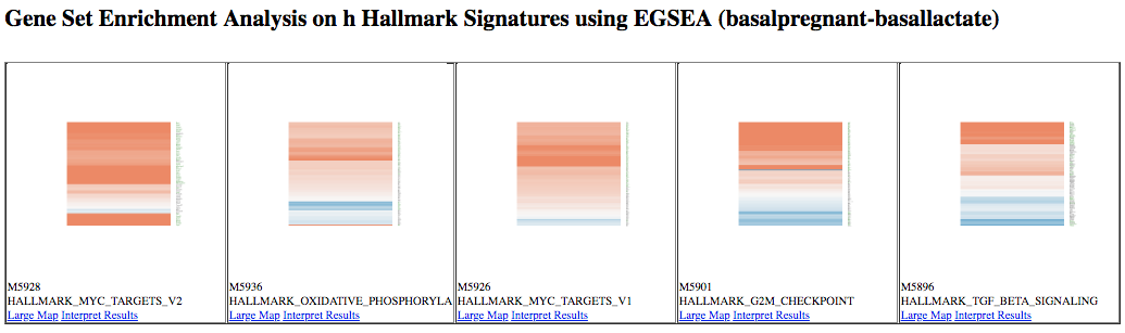
This generates a table of results, and a report. Contained within the report are plots, such as heatmaps of the top ranked pathways, as shown below. Note that we see some similar pathways in the results here as with the fgsea analysis.
KEGG pathway diagrams are generated if KEGG pathways are selected, as shown below. These show the expression values of the genes overlaid, genes upregulated in the contrast are shown in red, downregulated genes in blue. Ribosome was one of the top GO terms identified for the basal pregnant vs lactate contrast and here we see ribosome pathways are in the top ranked KEGG pathways.
Can you run EGSEA on the luminal contrast identify the top KEGG gene sets? Tip: you could use the rerun button and replace the “Contrast of Interest” with the name of the luminal contrast.
Running EGSEA on the luminal file should give top KEGG gene sets similar to below.
In this tutorial we have seen some gene set testing methods that can be used to interpret lists of differentially expressed genes. Multiple methods can be used to help identify pathways of interest and to provide complementary ways of visualising results. This follows on from the accompanying tutorials, RNA-seq reads to counts and RNA-seq counts to genes, that showed how to turn reads (FASTQs) into differentially expressed genes for this dataset. For further reading on analysis of RNA-seq count data and the methods used here, see the articles; RNA-seq analysis is easy as 1-2-3 with limma, Glimma and edgeR (Law et al. 2016) and From reads to genes to pathways: differential expression analysis of RNA-Seq experiments using Rsubread and the edgeR quasi-likelihood pipeline (Chen, Lun, Smyth 2016).
You've Finished the Tutorial
Please also consider filling out the Feedback Form as well!
Key points
goseq can be used to identify enriched gene ontology categories and incorporate gene length bias
fgsea can be used to identify enriched gene sets, such as the MSigDB collections, and generate barcode plots
EGSEA can be used to identify enriched gene sets, such as MSigDB and KEGG, generating visualisations that include heatmaps and KEGG pathway diagrams
Multiple methods can be used to help identify differentially expressed pathways and to visualise results
Frequently Asked Questions
Have questions about this tutorial? Have a look at the available FAQ pages and support channels
Further information, including links to documentation and original publications, regarding the tools, analysis techniques and the interpretation of results described in this tutorial can be found here.
Feedback
Did you use this material as an instructor? Feel free to give us feedback on how it went.
Did you use this material as a learner or student? Click the form below to leave feedback.
Hiltemann, Saskia, Rasche, Helena et al., 2023 Galaxy Training: A Powerful Framework for Teaching! PLOS Computational Biology 10.1371/journal.pcbi.1010752
Batut et al., 2018 Community-Driven Data Analysis Training for Biology Cell Systems 10.1016/j.cels.2018.05.012
@misc{transcriptomics-rna-seq-genes-to-pathways,
author = "Maria Doyle and Belinda Phipson",
	title = "3: RNA-seq genes to pathways (Galaxy Training Materials)",
	year = "",
	month = "",
	day = "",
	url = "\url{https://training.galaxyproject.org/training-material/topics/transcriptomics/tutorials/rna-seq-genes-to-pathways/tutorial.html}",
	note = "[Online; accessed TODAY]"
}
@article{Hiltemann_2023,
	doi = {10.1371/journal.pcbi.1010752},
	url = {https://doi.org/10.1371%2Fjournal.pcbi.1010752},
	year = 2023,
	month = {jan},
	publisher = {Public Library of Science ({PLoS})},
	volume = {19},
	number = {1},
	pages = {e1010752},
	author = {Saskia Hiltemann and Helena Rasche and Simon Gladman and Hans-Rudolf Hotz and Delphine Larivi{\`{e}}re and Daniel Blankenberg and Pratik D. Jagtap and Thomas Wollmann and Anthony Bretaudeau and Nadia Gou{\'{e}} and Timothy J. Griffin and Coline Royaux and Yvan Le Bras and Subina Mehta and Anna Syme and Frederik Coppens and Bert Droesbeke and Nicola Soranzo and Wendi Bacon and Fotis Psomopoulos and Crist{\'{o}}bal Gallardo-Alba and John Davis and Melanie Christine Föll and Matthias Fahrner and Maria A. Doyle and Beatriz Serrano-Solano and Anne Claire Fouilloux and Peter van Heusden and Wolfgang Maier and Dave Clements and Florian Heyl and Björn Grüning and B{\'{e}}r{\'{e}}nice Batut and},
	editor = {Francis Ouellette},
	title = {Galaxy Training: A powerful framework for teaching!},
	journal = {PLoS Comput Biol}
}
Congratulations on successfully completing this tutorial!
You can use Ephemeris's shed-tools install command to install the tools used in this tutorial.
5 stars:
Liked: really liked being able to use multiple methods to generate enrichment analysis
5 stars:
Liked: agin step by step, very clear
September 2025
5 stars:
Liked: How the tutorial flows. It's well written and put together.
Disliked: There are new versions of the software used in this tutorial. Please go through and edit the tutorial. Some options changed and it took some tinkering around to make sure I got the programs working.
January 2025
4 stars:
Liked: For the most part, the instructions were easy to follow-- what tools to use and where was extremely clear
Disliked: Specifically in formatting the files for goseq, it would be helpful to have some reference point for what the input files should look like so that this tutorial can be applied to datasets beyond those provided. For example, in the portion of the tutorial where you add a bool(c8<0.01) column to help prepare the goseq inputs, it's unclear where in the tabular file that column should be added because the tool prompts you to pick where in the file to insert the new column (do you append it to the existing file? insert an entirely new column? And if inserted, then where?)
August 2024
3 stars:
Liked: The process was well described.
Disliked: However, how we can do the "Functional enrichment analysis of the DE genes" on genomes other than humans or mice is not explained.
December 2023
5 stars:
Liked: It was explicit and clear
Disliked: Please show wich versions of plugins and software ur using
June 2023
1 stars:
Liked: Misleading and poor
November 2022
5 stars:
Liked: The fact that from nothing i can do RNA sequencing from start to bottom
Disliked: Maybe tutorials with other tools from galaxy
5 stars:
Liked: Hands on data analysis, problem solving
Disliked: maybe notification of different tools with similar names? but really I guess it was fun problem solving
November 2020
4 stars:
Liked: Everything worked and the steps didn't take too much time. ALso It was good to see the luminal data used. I don't think it was used in the prvious tutorials (although it may have been an option - I'll double check.) We did it any way.
Disliked: I'd like to see more discussion of what to make of these gene and process lists. The first go method came up with categories such as "cell" what to make of this? Also - the gene lists identified in these tutorials does not match that of the Fu paper. Probably because a smaller data set was used ?
October 2019
5 stars:
Liked: very clear, good sample data
August 2019
5 stars:
Liked: easy to follow. thank you for including a picture of the results for comparison
Disliked: more analysis/interpretation
Questions:
 Open image in new tab


 Open image in new tab
Open image in new tab
 Open image in new tab
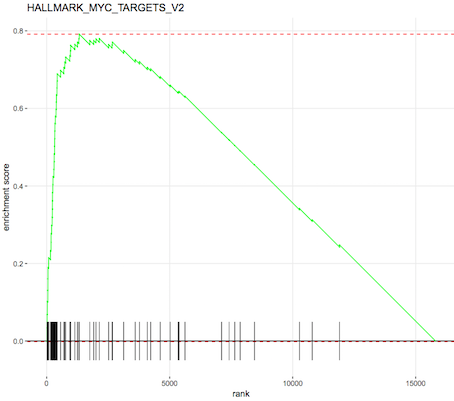 Open image in new tab
Open image in new tab
 Open image in new tab
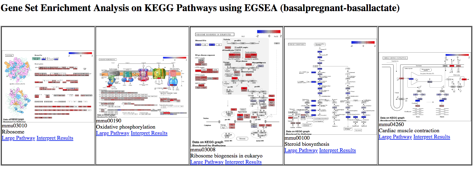 Open image in new tab
Open image in new tab
