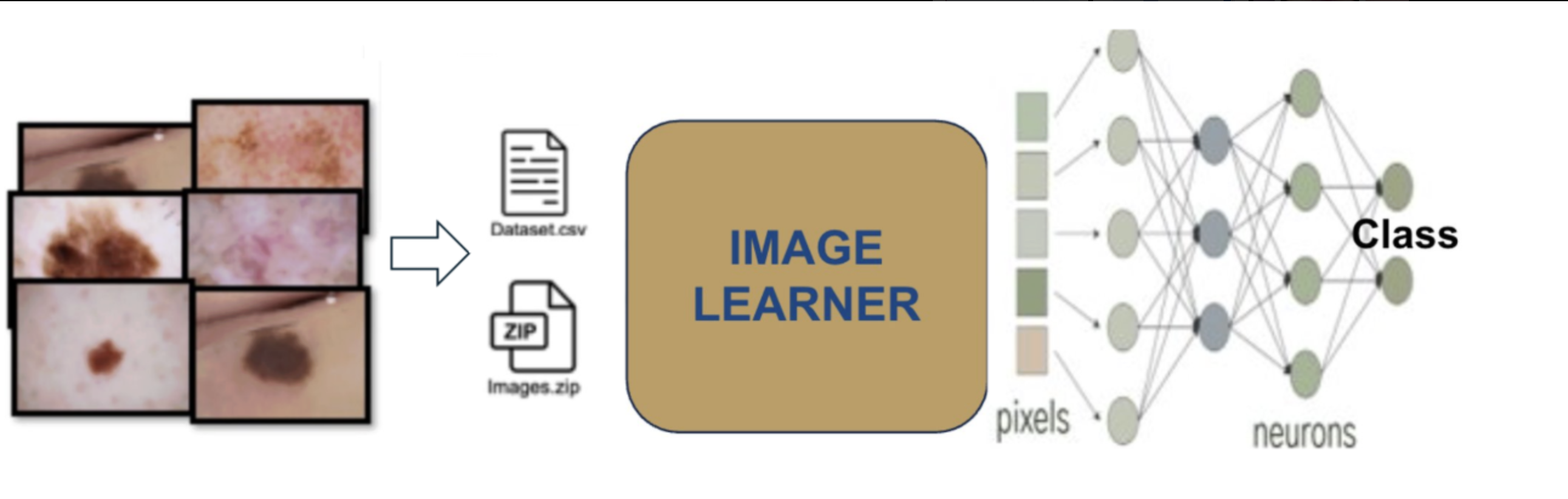
In this tutorial, we will use the HAM10000 (“Human Against Machine with 10,000 training images”) dataset to develop a deep learning classifier for dermoscopic skin lesion classification. The goal is to accurately classify seven types of pigmented skin lesions using the GLEAM Image Learner tool.
To achieve this, we will follow three essential steps: (i) upload the HAM10000 images and metadata to Galaxy, (ii) set up and run the Image Learner tool to train a deep learning model, and (iii) evaluate the model’s predictive performance by analyzing key performance metrics such as accuracy, ROC-AUC, and confusion matrices.
The HAM10000 dataset is a preprocessed subset of the original HAM10000 collection, following the methodology described by Shetty et al. 2022. The dataset covers seven types of pigmented skin lesions:
Melanoma (mel)
Melanocytic nevus (nv)
Basal cell carcinoma (bcc)
Actinic keratosis (akiec)
Benign keratosis (bkl)
Dermatofibroma (df)
Vascular lesion (vasc)
To address class imbalance in the original dataset, we applied preprocessing steps.
Dataset Preprocessing and Composition
The dataset used in this tutorial has been preprocessed following the methodology from Shetty et al. 2022 to create a balanced training set suitable for deep learning.
Preprocessing Steps
Starting from the original HAM10000 dataset (10,015 images with severe class imbalance), we applied the following preprocessing:
Step 1: Image Selection
Selected 100 images per class from the original dataset
Ensured balanced representation across all 7 lesion types
Step 2: Image Resizing
Resized all images to 96×96 pixels
Standardized format as PNG for consistent processing
Step 3: Data Augmentation
Applied horizontal flip augmentation to each image
Generated 200 images per class (100 original + 100 flipped)
Total dataset: 1,400 images (200 × 7 classes)
This preprocessing addresses the severe class imbalance in the original HAM10000 dataset where melanocytic nevi represented 67% of images while dermatofibroma represented only 1.1%.
Balanced Dataset Composition
The preprocessed dataset provides balanced representation:
Lesion Type
Images
Percentage
Melanocytic nevus (nv)
200
14.3%
Melanoma (mel)
200
14.3%
Basal cell carcinoma (bcc)
200
14.3%
Actinic keratosis (akiec)
200
14.3%
Benign keratosis (bkl)
200
14.3%
Dermatofibroma (df)
200
14.3%
Vascular lesion (vasc)
200
14.3%
Total
1,400
100%
This balanced dataset allows the Image Learner model to learn effectively from all lesion types without bias toward the majority class.
Metadata Columns (HAM10000 CSV)
The metadata CSV now includes additional fields while keeping the same number of samples and the same flip augmentation strategy. Each row corresponds to one image file.
Column
Description
lesion_id
Lesion identifier used to group original and augmented images from the same lesion.
image_id
Image identifier from the source dataset (shared by original and flipped versions).
dx
Diagnosis label (target class).
dx_type
Diagnosis confirmation method (for example, histo).
age
Patient age in years.
sex
Patient sex (male/female/unknown).
localization
Anatomical site of the lesion.
image_path
Image filename within the image ZIP.
Following the preprocessing pipeline described by Shetty et al. 2022, horizontal flip augmentation is applied during dataset preparation. Horizontal flips:
Improve robustness to lesion orientation and acquisition variability
Increase effective training diversity without collecting additional images
Help reduce sensitivity to class- and pose-specific patterns
Preserve diagnostically relevant structures while introducing harmless variation
In Shetty et al. 2022, this preprocessing strategy (including horizontal flips) is associated with improved HAM10000 skin-lesion classification performance (reported accuracy: 95.18%).
Click galaxy-uploadUpload at the top of the activity panel
Select galaxy-wf-editPaste/Fetch Data
Paste the link(s) into the text field
Press Start
Close the window
For the .zip file, set the datatype to zip
For the .csv file, leave as Auto-Detect (it will be recognized as tabular)
Check that the data formats are assigned correctly:
The .zip file should have type zip
The .csv file should have type tabular
If they are not, follow the Changing the datatype tip:
Click on the galaxy-pencilpencil icon for the dataset to edit its attributes
In the central panel, click galaxy-chart-select-dataDatatypes tab on the top
In the galaxy-chart-select-dataAssign Datatype, select datatypes from “New Type” dropdown
Tip: you can start typing the datatype into the field to filter the dropdown menu
Click the Save button
Add tags to the datasets for better organization:
Add tag HAM10000_images to the skin_image.zip file
Add tag HAM10000_metadata to the image_metadata_new.csv file
Datasets can be tagged. This simplifies the tracking of datasets across the Galaxy interface. Tags can contain any combination of letters or numbers but cannot contain spaces.
To tag a dataset:
Click on the dataset to expand it
Click on Add Tagsgalaxy-tags
Add tag text. Tags starting with # will be automatically propagated to the outputs of tools using this dataset (see below).
Press Enter
Check that the tag appears below the dataset name
Tags beginning with # are special!
They are called Name tags. The unique feature of these tags is that they propagate: if a dataset is labelled with a name tag, all derivatives (children) of this dataset will automatically inherit this tag (see below). The figure below explains why this is so useful. Consider the following analysis (numbers in parenthesis correspond to dataset numbers in the figure below):
a set of forward and reverse reads (datasets 1 and 2) is mapped against a reference using Bowtie2 generating dataset 3;
dataset 3 is used to calculate read coverage using BedTools Genome Coverageseparately for + and - strands. This generates two datasets (4 and 5 for plus and minus, respectively);
datasets 4 and 5 are used as inputs to Macs2 broadCall datasets generating datasets 6 and 8;
datasets 6 and 8 are intersected with coordinates of genes (dataset 9) using BedTools Intersect generating datasets 10 and 11.
Now consider that this analysis is done without name tags. This is shown on the left side of the figure. It is hard to trace which datasets contain “plus” data versus “minus” data. For example, does dataset 10 contain “plus” data or “minus” data? Probably “minus” but are you sure? In the case of a small history like the one shown here, it is possible to trace this manually but as the size of a history grows it will become very challenging.
The right side of the figure shows exactly the same analysis, but using name tags. When the analysis was conducted datasets 4 and 5 were tagged with #plus and #minus, respectively. When they were used as inputs to Macs2 resulting datasets 6 and 8 automatically inherited them and so on… As a result it is straightforward to trace both branches (plus and minus) of this analysis.
After uploading the dataset, configure the Image Learner parameters as follows. These settings are based on best practices for dermoscopic image classification and have been optimized for the HAM10000 dataset.
Hands On: Configure Image Learner for HAM10000
Image Learner ( Galaxy version 0.1.5) with the following parameters:
Stop when validation metrics stall to avoid overfitting
Fine Tune
True
Leverage pre-trained features for better performance
Use Pretrained
True
Transfer learning from ImageNet-trained weights
Learning Rate
0.001
Conservative learning rate for fine-tuning
Random Seed
42
Reproducible results across runs
Data Split
70/10/20
Standard split for training/validation/test (automatically applied when no split column exists in metadata CSV)
Data Augmentation
Horizontal and Vertical Flip; Rotate; Blur; Brightness; Contrast
Improve generalization
The Image Learner tool automatically applies a stratified 70/10/20 train/validation/test split by default when no split column is present in the metadata CSV file. Per-class counts can differ by a few samples due to rounding. This ensures balanced representation of all classes across the three datasets. The stratified split maintains the same class distribution in each split, which is particularly important for imbalanced datasets. If you want to use a custom split, you can add a split column to your metadata CSV with values 0 (train), 1 (validation), or 2 (test).
After training and testing your model, you should see several new files in your history list:
Image Learner Trained Model (ludwig_model): A reusable model bundle that includes the model configuration JSONs and model weights.
Image Learner Model Report (HTML): An interactive report that summarizes configuration, metrics, and plots.
Image Learner Predictions/Stats/Plots (collection): A list collection containing:
predictions.csv with model predictions and confidence scores
JSON files (for example training_statistics.json, test_statistics.json, description.json) with experiment metadata and metrics
PNG plots from visualizations/train and visualizations/test, plus feature importance example images
feature_importance_examples.zip bundling the feature importance examples
For this tutorial, we will focus on the Image Learner Model Report and the performance metrics.
Image Learner Model Report
The Image Learner HTML report provides a comprehensive and interactive overview of the trained model’s performance. It is organized into three tabs that separate configuration, training/validation diagnostics, and test results.
Config and Overall Performance Summary
This tab combines dataset composition, overall metrics, and configuration details:
Dataset Overview: Sample counts per class and split (train/validation/test). For regression tasks, only split counts are shown.
Model Performance Summary: A sortable table of metrics across train, validation, and test splits.
Training Configuration: Model architecture, image size, augmentation, split strategy, optimizer, learning rate, epochs, early stopping, and random seed.
Metrics Help: A “Help” button that opens a glossary explaining each metric.
These weighted metrics indicate balanced performance across classes under the explicitly balanced split. The report also includes ROC-AUC and Cohen’s Kappa for additional discrimination and agreement context.
Per-class Metrics
The report summarizes performance for each lesion class using a heatmap of key classification metrics. Rows correspond to classes (e.g., akiec, bcc, bkl, df, mel, nv, vasc) and columns correspond to evaluation metrics. Darker cells indicate stronger performance (values closer to 1.0).
Precision: of the images predicted as a class, how many are correct (higher = fewer false positives).
Recall: of the true images of a class, how many were found (higher = fewer false negatives).
F1 score: balance of precision and recall.
Accuracy: class-wise correctness under the one-vs-rest view reported by the tool.
Matthews correlation coefficient (MCC): correlation-style score robust to class imbalance (higher is better).
Specificity: how well the model avoids labeling other classes as this class (higher = fewer false positives).
Use this view to quickly spot classes that are consistently strong across metrics (darker row) versus classes where performance lags in specific dimensions (lighter cells), guiding targeted follow-ups (e.g., more data, label review, or augmentation).
The confusion matrix provides a detailed breakdown of correct and incorrect predictions for each class, highlighting which lesion types are most frequently confused.
Image Learner shows slightly lower accuracy (0.88 vs. 0.94) but higher weighted precision/recall/F1 (0.90 vs. 0.88/0.85/0.86).
The balanced split comparison aligns with the published benchmark and shows strong weighted metrics under the same evaluation style.
The leakage-aware split provides a more conservative, realistic estimate by keeping original and flipped images from the same lesion together.
Image Learner provides publication-ready metrics and visualizations with full reproducibility through Galaxy.
Tutorial takeaways
The Image Learner comparison is competitive with the published CNN benchmark on the balanced HAM10000 subset.
Leakage-aware splitting prevents inflated performance and is essential when augmentations create near-duplicate images.
The tool makes it easy to enforce leakage-aware splits while keeping diagnostics transparent and reproducible.
Conclusion
In this tutorial, we used the Galaxy Image Learner tool to build and evaluate a dermoscopic lesion classifier on the HAM10000 dataset with a balanced split and a CaFormer backbone:
Upload the images and metadata.
Configure and train the model.
Review test metrics and diagnostic plots, and compare results to the Shetty et al. benchmark.
The model achieved ~88% accuracy with balanced weighted precision/recall/F1 of ~0.90 under the balanced split, and ~0.66 across metrics under the leakage-aware split. These steps generalize to other biomedical image-classification tasks while highlighting the importance of leakage-aware evaluation.
You've Finished the Tutorial
Please also consider filling out the Feedback Form as well!
Key points
Use Galaxy tools (Image Learner) to build a deep learning model for skin lesion classification based on the HAM10000 dataset.
Understand the dataset composition and the importance of data augmentation to handle class imbalance.
Confirm the robustness of the model by evaluating its performance metrics including accuracy, ROC-AUC, and F1-score.
Frequently Asked Questions
Have questions about this tutorial? Have a look at the available FAQ pages and support channels
Shetty, B., R. Fernandes, A. P. Rodrigues, R. Chengoden, S. Bhattacharya et al., 2022 Skin lesion classification of dermoscopic images using machine learning and convolutional neural network. Scientific Reports 12: 10.1038/s41598-022-22644-9
Feedback
Did you use this material as an instructor? Feel free to give us feedback on how it went.
Did you use this material as a learner or student? Click the form below to leave feedback.
Hiltemann, Saskia, Rasche, Helena et al., 2023 Galaxy Training: A Powerful Framework for Teaching! PLOS Computational Biology 10.1371/journal.pcbi.1010752
Batut et al., 2018 Community-Driven Data Analysis Training for Biology Cell Systems 10.1016/j.cels.2018.05.012
@misc{statistics-image_learner,
author = "Khai Van Dang and Paulo Cilas Morais Lyra Junior and Junhao Qiu and Alyssa Pybus and Jeremy Goecks",
	title = "GLEAM Image Learner - Validating Skin Lesion Classification on HAM10000 (Galaxy Training Materials)",
	year = "",
	month = "",
	day = "",
	url = "\url{https://training.galaxyproject.org/training-material/topics/statistics/tutorials/image_learner/tutorial.html}",
	note = "[Online; accessed TODAY]"
}
@article{Hiltemann_2023,
	doi = {10.1371/journal.pcbi.1010752},
	url = {https://doi.org/10.1371%2Fjournal.pcbi.1010752},
	year = 2023,
	month = {jan},
	publisher = {Public Library of Science ({PLoS})},
	volume = {19},
	number = {1},
	pages = {e1010752},
	author = {Saskia Hiltemann and Helena Rasche and Simon Gladman and Hans-Rudolf Hotz and Delphine Larivi{\`{e}}re and Daniel Blankenberg and Pratik D. Jagtap and Thomas Wollmann and Anthony Bretaudeau and Nadia Gou{\'{e}} and Timothy J. Griffin and Coline Royaux and Yvan Le Bras and Subina Mehta and Anna Syme and Frederik Coppens and Bert Droesbeke and Nicola Soranzo and Wendi Bacon and Fotis Psomopoulos and Crist{\'{o}}bal Gallardo-Alba and John Davis and Melanie Christine Föll and Matthias Fahrner and Maria A. Doyle and Beatriz Serrano-Solano and Anne Claire Fouilloux and Peter van Heusden and Wolfgang Maier and Dave Clements and Florian Heyl and Björn Grüning and B{\'{e}}r{\'{e}}nice Batut and},
	editor = {Francis Ouellette},
	title = {Galaxy Training: A powerful framework for teaching!},
	journal = {PLoS Comput Biol}
}
Congratulations on successfully completing this tutorial!
You can use Ephemeris's shed-tools install command to install the tools used in this tutorial.
Questions:
 Open image in new tab
Open image in new tab


 Open image in new tab
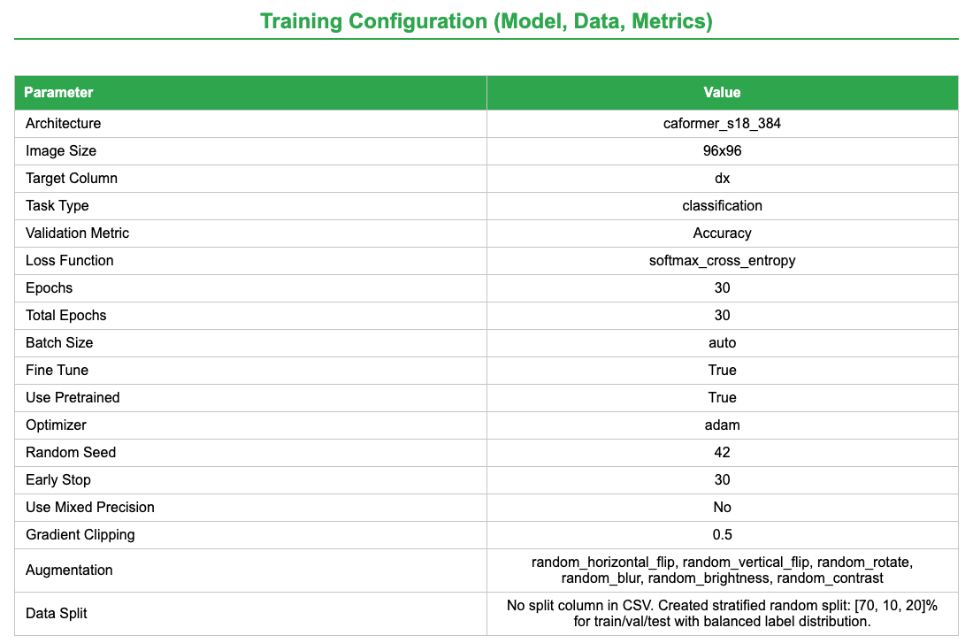 Open image in new tab
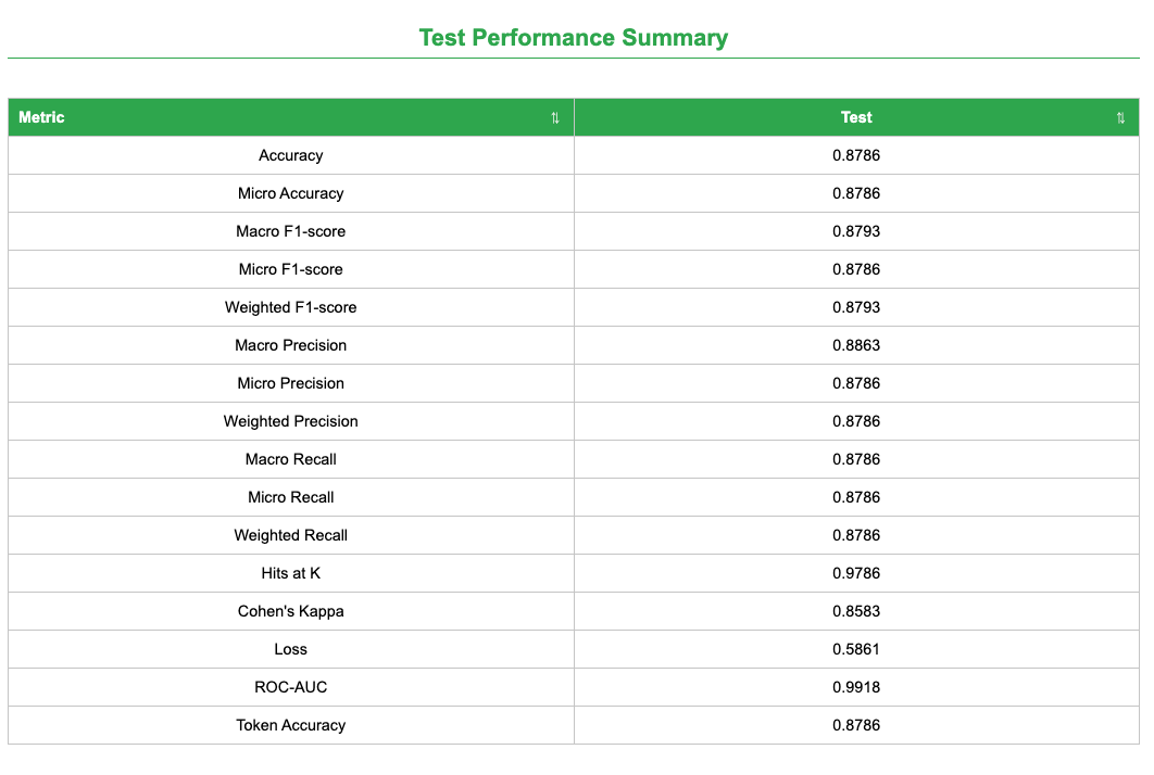 Open image in new tab
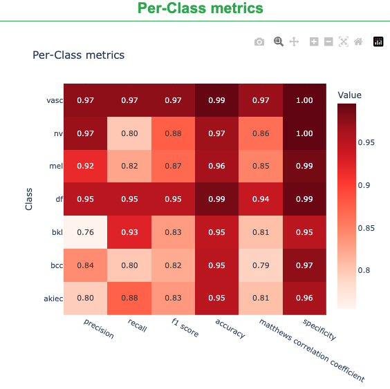 Open image in new tab
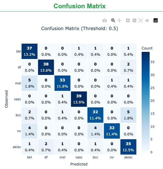 Open image in new tab
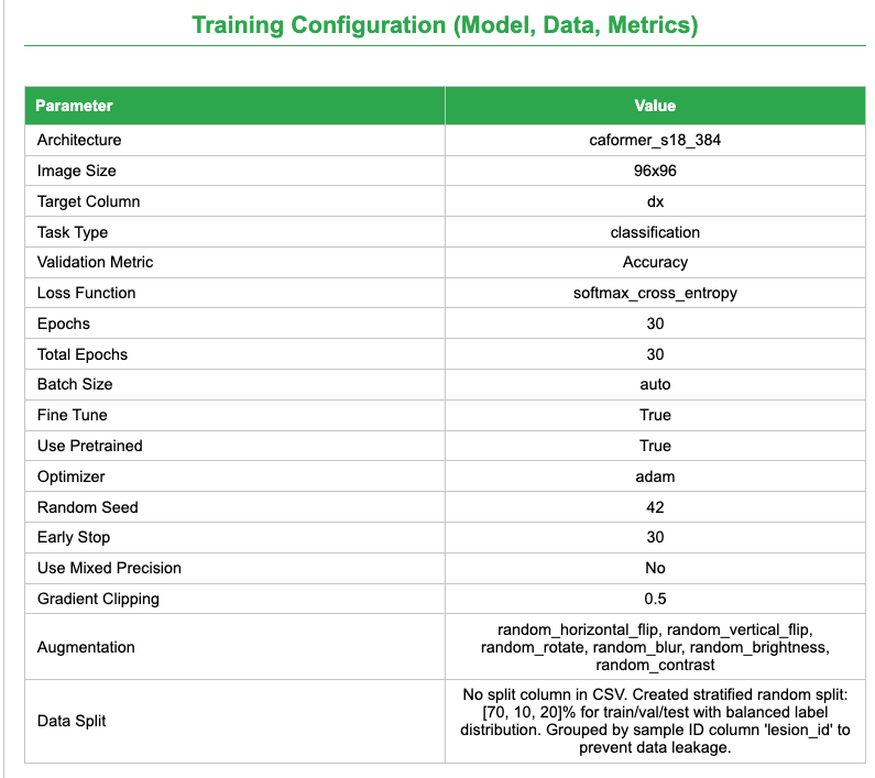 Open image in new tab
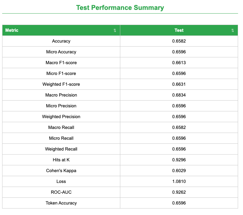 Open image in new tab