In microbiology, identifying links between genotype and phenotype is key to understand bacteria growth and virulence mechanisms, and to identify targets for drugs and vaccines. These analysis are limited by the lack of bacterial genome annotations (e.g. 30% of genes for S. pneumoniae are of unknown function) and by the fact that genotypes often arose from complex composant interactions.

Transposon insertion Sequencing

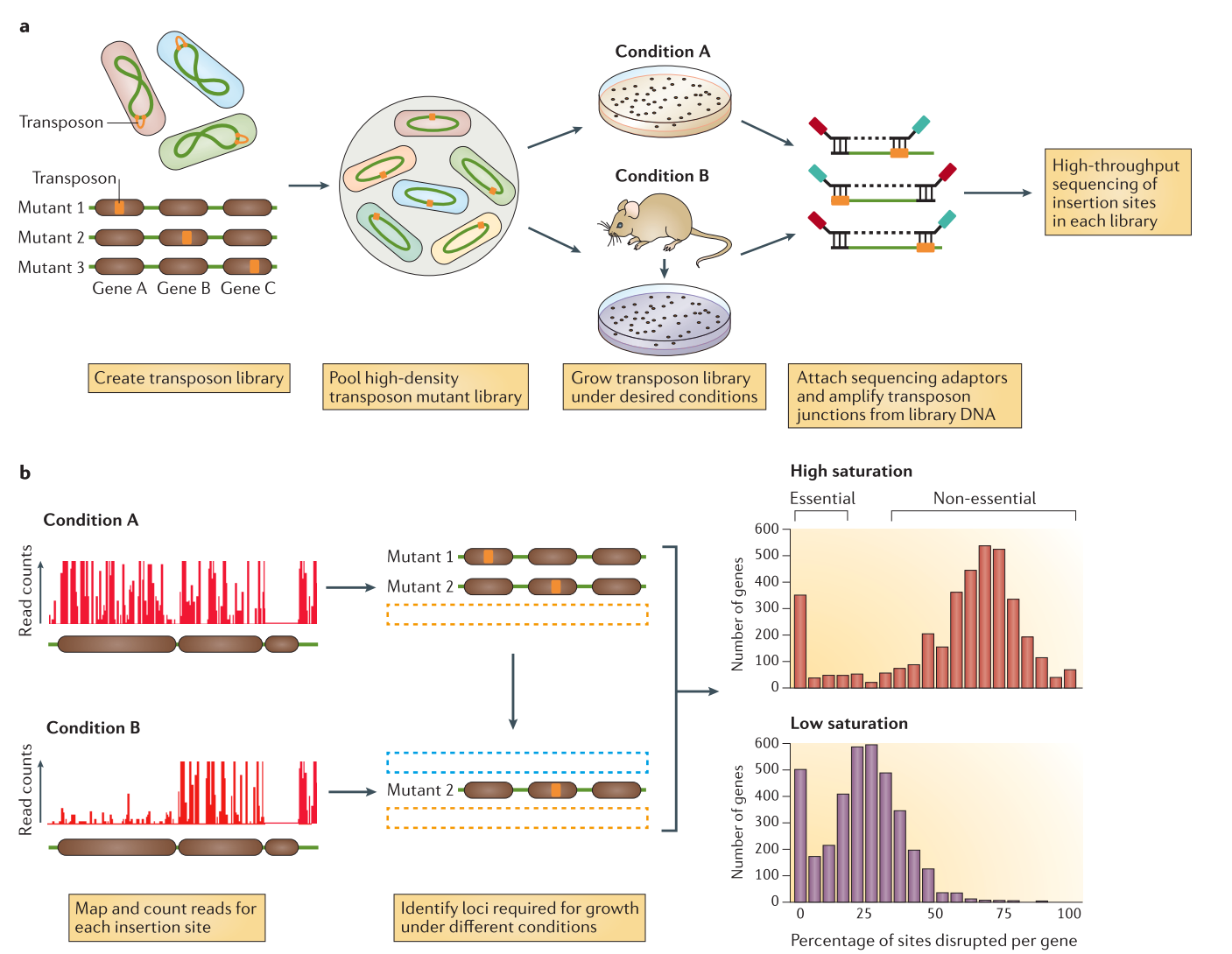
Transposon insertion sequencing is a technique used to functionally annotate bacterial genomes. In this technique, the genome is saturated by insertions of transposons. Transposons are highly regulated, discrete DNA segments that can relocate within the genome. They have a large influence on gene expression and can be used to determine the function of genes.

When a transposon inserts itself in a gene, the gene’s function will be disrupted, affecting the fitness (growth) of the bacteria. We can then manipulate transposons for use in insertional mutagenesis, i.e. creation of mutations of DNA by the addition of transposons. The genomes can be then sequenced to locate the transposon insertion site and the function affected by a transposon insertion can be linked to the disrupted gene.

Open image in new tab

1. Data production (a in the previous image)

   An initial population of genomes is mutated so that the genome of the bacteria is saturated with transposon insertions. A library is called saturated if in the genomes across the whole population of bacteria, each potential insertion site has at least one insertion. The population is then divided into several media containing different growth conditions, to identify the impact of the insertions on the bacteria growth. After growth, the regions flanking the insertion are amplified and sequenced, allowing to determine the location of the insertion.

2. Analysis (b in the previous image)

   The sequences are aligned to the reference genome to identify the location of the regions flanking the insertions. The resulting data will show a discrete repartition of reads on each site. If a gene present several insertions, like the two leftmost genes in Condition A, it means that its disruption has little or no impact to the bacterial growth. On the other hand, when a gene shows no insertions at all, like the rightmost gene in Condition A, is means that any disruption in this gene killed the bacteria, meaning it is a gene essential to bacteria survival. If the library is sufficiently saturated, there is a clear threshold between essential and non-essential genes when you analyze the insertion rate per gene.

Two type of transposon insertion methods exist:

• Gene disruption, where we analyze only the disruptions. This will covered by of this tutorial
• Regulatory element insertion, where different promoters are inserted by the transposon, and we analyze the change in gene expression in addition to the disruption. This method will be the subject of another tutorial.

Building a TnSeq library

Different types of transposons can be used depending of the goal of your analysis.

• Randomly pooled transposon

  • Mariner-based transposons, common and stable transposons which target the “TA” dinucleotides

    The TA are distributed relatively evenly along genome. The Mariner-based transposons can be inserted to impact statistically every gene, with in average more than 30 insertions site per kb. With the low insertion bias, it is easy to build saturated libraries. But local variations means less loci and less statistical power.

  • Tn5-based vectors, which insert at random sites

    This transposon do not require any target sequences. It is useful for specie where it is difficult to build mariner based transposons. But it has a preference for high GC content, causing insertion bias

• Defined sequence transposon

  It can be used to study interactions in pathways of interest, but also more precise targeting (small genes, pathways) for specific analyses

Independently of the transposon choice we need to be careful about the library complexity. With a large complex library, multiple insertion can be found in every potential locus. The higher density of insertion, the greater precision in identifying limits of regions of interest. If the density of the library is too low, some genes might by chance not be disrupted and mistaken for essential. The advantage of a target specific transposon, like the mariner, in opposition of a Tn5-based transposon inserting randomly, it that the limited number of insertion sites makes it easier to build high complexity libraries.

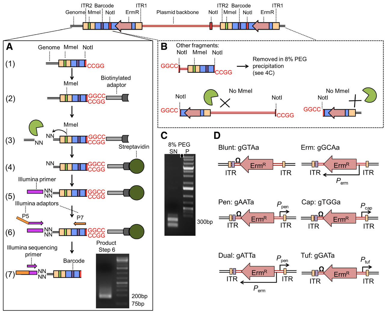
After selection of the type of transposon, we need to modify it to allow insertion site amplification and sequencing to get a library fitting the transposon insertion. Biases could be introduced during the process due to uneven fragment sizes. To avoid that, we can introduce a Type I restriction site to cleave DNA downstream of transposon, and get uniform fragment sizes and therefore avoid a bias in the representation of the insertions.

As we just want to identify the TA site affected by an insertion, we only need the location of the start of the reads and not a good coverage of the entire genome. Long reads are then not so important. On the other hand, a minimum transposon length of 16 bp is necessary for precise mapping on the genome Kwon et al. 2015. We can therefore not use the BsmFI restriction site (11 to 12 bp) but MmeI.

In this tutorial, we are using mariner transposon targeting TA sequences, in ordered to target the whole genome uniformly, with two specific regions used to specifically sequence the region upstream of the insertion Santiago et al. 2015

Open image in new tab

The transposon inserts itself at TA site at the ITR junctions. These ITR junctions have been modified to include a Mme1 restriction site and a NotI restriction site which cut 21 bp upstream the restriction site. These two site are the 5’ and 3’ limits to the genomic DNA we want to sequence.

1. After digestion by NotI restriction enzyme, the fragments are attached to biotinylated adaptors that link to NotI restriction site. The attached fragment are then digested by MMeI at a site upstream, where an Illumina primer is then linked. The sequencing is then done, adding Illumina adaptors and an additional barcode to the read for multiplexed sequencing.

2. An insertion can sometimes be composed of one or more copies of the transposon (multimer). There is therefore a risk to select plasmid backbone sequence. To solve this problem, an additional NotI has been added in the backbone to create different length construct, that can later be filtrated. Different promoters are added with an additional 3 bp barcode to analyze differential expression impact. This type of complex analysis will be covered in a follow-up tutorial.

Because of this complex transposon structure, the reads obtained after sequencing contain a lot of adapters and foreign sequences used to insert and target the transposon. Several steps of preprocessing are then need to extract only the transposon sequence before finding its location on the genome.

Tnseq analysis

Once the genomic sequences are extracted from the initial reads (i.e. remove non genomic sequences from the reads), they need to be located each on the genome to link them to a TA site and genes. To do that we map them to a reference genome, link them to a specific insertion site, and then count the number of insertion for each TA site and identify essential genes of regions.

We will apply this approach in this tutorial using a subset of TnSeq reads from Santiago et al. 2015.

Agenda

In this tutorial, we will deal with:

1. Transposon insertion Sequencing
2. Building a TnSeq library
3. Tnseq analysis
4. Data upload
5. Remove all non genomic sequences from the sequenced reads
   1. Separate reads by experimental conditions
   2. Remove Adapter sequence
   3. Separate reads from different transposon constructs
   4. Remove the remaining transposon sequence
6. Count the number of insertion per TA sites
   1. Align the reads to a reference genome
   2. Compute coverage of the genome
   3. Identify TA sites positions
   4. Merge overall coverage and positions of TA sites to get the coverage of each TA sites
7. Predicting Essential Genes with Transit
   1. Transit
   2. Predict the essentiality of genes
   3. Compare the essential genes between two conditions
8. Conclusion

Data upload

Let’s start with uploading the data.

Hands-on: Import the data

1. Create a new history for this tutorial and give it a proper name

   Tip: Creating a new history

   To create a new history simply click the new-history icon at the top of the history panel:

   

   Tip: Renaming a history

   1. Click on galaxy-pencil (Edit) next to the history name (which by default is “Unnamed history”)
   2. Type the new name
   3. Click on Save
   4. To cancel renaming, click the galaxy-undo “Cancel” button

   If you do not have the galaxy-pencil (Edit) next to the history name (which can be the case if you are using an older version of Galaxy) do the following:

   1. Click on Unnamed history (or the current name of the history) (Click to rename history) at the top of your history panel
   2. Type the new name
   3. Press Enter

2. Import from Zenodo or a data library (ask your instructor):
   • FASTQ file with the Tnseq reads: Tnseq-Tutorial-reads.fastqsanger.gz
   • Set of barcodes to separate reads from different experimental conditions: condition_barcodes.fasta
   • Set of barcodes to separate reads from different transposon constructs: construct_barcodes.fasta
   • Genome file for Staphylococcus aureus: staph_aur.fasta
   • Annotation file for Staphylococcus aureus: staph_aur.gff3

   https://zenodo.org/record/2579335/files/Tnseq-Tutorial-reads.fastqsanger.gz
   https://zenodo.org/record/2579335/files/condition_barcodes.fasta
   https://zenodo.org/record/2579335/files/construct_barcodes.fasta
   https://zenodo.org/record/2579335/files/staph_aur.fasta
   https://zenodo.org/record/2579335/files/staph_aur.gff3
   

   Tip: Importing via links

   • Copy the link location

   • Click galaxy-upload Upload Data at the top of the tool panel

   • Select galaxy-wf-edit Paste/Fetch Data

   • Paste the link(s) into the text field

   • Press Start

   • Close the window

   Tip: Importing data from a data library

   As an alternative to uploading the data from a URL or your computer, the files may also have been made available from a shared data library:

   1. Go into Data (top panel) then Data libraries
   2. Navigate to the correct folder as indicated by your instructor.
      • On most Galaxies tutorial data will be provided in a folder named GTN - Material –> Topic Name -> Tutorial Name.
   3. Select the desired files
   4. Click on Add to History galaxy-dropdown near the top and select as Datasets from the dropdown menu

   5. In the pop-up window, choose

      • “Select history”: the history you want to import the data to (or create a new one)
   6. Click on Import

3. Rename the files

   Tip: Renaming a dataset

   • Click on the galaxy-pencil pencil icon for the dataset to edit its attributes
   • In the central panel, change the Name field
   • Click the Save button

Remove all non genomic sequences from the sequenced reads

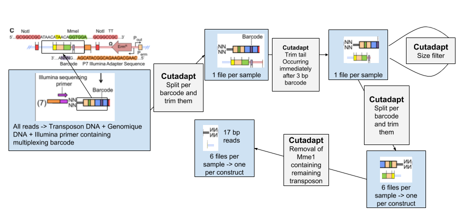
Because of the experimental design for transposon insertion sequencing, the raw reads contain a lot of adapters and foreign sequences used to insert and target the transposon. To obtain the core reads that contain only genomic sequence, the reads have to go through several steps (using the Cutadapt tool) to remove them and divide the reads per experimental condition and type of transposon:

Open image in new tab

1. We separate the reads of each experimental condition based on a 8 bp barcode at the beginning of each read. These barcodes were added to be able to pool different conditions together before the transposon insertion and sequencing.
2. The tail of each set of read is then removed. It immediately follows the 3 bp barcode specific to transposon constructs, and contains illumina adapter sequence and downstream
3. To be sure all our reads have been trimmed correctly we filter out the reads too large.
4. We then separate the reads per transposon construct
5. We remove the remaining transposon sequence containing MmeI.

Separate reads by experimental conditions

First we divide the initial data set by experimental conditions using the 8 bp barcode added during the Illumina multiplexing protocol.

Hands-on: Inspect condition barcodes

1. Inspect the condition_barcodes file

This fasta file contains the barcodes for each condition:

>control
^CTCAGAAG
>condition
^GACGTCAT

We can see 2 barcodes there: one for control and one for condition.

Comment: Barcode symbols used by Cutadapt

The ^ at the beginning of the sequence means we want to anchor the barcode at the beginning of the read. To know more about the symbols used by Cutadapt, you check the Cutadapt manual.

We would like now to split our Tnseq reads in Tnseq-Tutorial-reads given the barcodes.

Hands-on: Split reads by condition barcodes using Cutadapt

1. Cutadapt tool with:
   • “Single-end or Paired-end reads?”: Single-end
     • param-file “FASTQ/A file”: Tnseq-Tutorial-reads
     • In “Read 1 Options”
       • In “5’ (Front) Adapters”
         • Click on “Insert 5’ (Front) Adapters”
           • “Source”: File From History
             • “Choose file containing 5’ adapters”: condition_barcodes file
   • In “Adapter Options”
     • “Maximum error rate”: 0.15 (to allow 1 mismatch)
     • “Match times”: 3 (to cover cases where barcodes are attached several times)
   • In “Output Selector”, select
     • “Report”
     • “Multiple output” (to separate the reads into one file per condition)
     • “Untrimmed reads” (to write reads that do not contain the adapter to a separate file)

   The output is a collection of the different conditions datasets, here control and condition, and a report text file.

2. Inspect the report text generated by Cutadapt tool

Question

1. What percentage of reads has been trimmed for the adapter?
2. How many reads have been trimmed for each condition?
3. What should we change if our barcodes were at the end of the reads ?

Solution

1. 100% of the reads were trimmed (line Reads with adapters)
2. 2,847,018 for control (CTCAGAAG barcode) and 2,862,108 for condition (GACGTCAT barcode)
3. We should use the option “Insert 3’ (End) Adapters” and anchored them at the end of the read with the symbol $ in our fasta file containing the barcodes.

Remove Adapter sequence

Our reads are now divided by condition. We need to trim their tail containing the Illumina adapters, used for initiating the sequencing (CGTTATGGCACGC, here). To do so, we remove the adapter and everything downstream, using the end adapter option of Cutadapt and not anchor the sequence anywhere. To eliminate reads that might not have been trimmed because of too many mismatches or other reasons, we filter the reads by size, given the known approximate size of the remaining sequences (how is it computed??).

Hands-on: Remove Adapter with Cutadapt

1. Cutadapt tool to remove adapters with:
   • “Single-end or Paired-end reads?”: Single-end
     • param-collection “FASTQ/A file”: collection output of the previous Cutadapt
     • In “Read 1 Options”
       • In “3’ (End) Adapters”
         • Click on “Insert 3’ (End) Adapters”
           • “Source”: Enter custom Sequence
             • “Enter custom 3’ adapter sequence”: CGTTATGGCACGC
   • In “Adapter Options”
     • “Match times”: 3 (to cover cases where barcodes are attached several times)
   • In “Output Selector”, select
     • “Report”

   Question

   What are the outputs at this step?

   Solution

   The outputs are two collections: one containing the reads in both conditions, and one containing the Cutadapt reports for each condition.

2. Inspect the generated report files

   Question

   What percentage of the reads contained the adapter?

   Solution

   More than 99% of the reads contained the adapter in both conditions (line Reads with adapters in the reports)

3. Cutadapt tool to filter reads based on length with:
   • “Single-end or Paired-end reads?”: Single-end
     • param-collection “FASTQ/A file”: collection output of the previous Cutadapt
   • In “Filter Options”
     • “Minimum length” : 64
     • “Maximum length” : 70
   • In “Output Selector”, select
     • “Report”

4. Inspect the generated report files

   Question

   How many reads where discarded after filtering?

   Solution

   Less than 2% of the reads were discarded in both conditions (lines Reads that were too short and Reads that were too long in the reports)

We can see that is both samples the reads have pass the filtering at more than 98%. If this percentage is very low, it means the previous trimming steps is incomplete or faulty.

Separate reads from different transposon constructs

The constructs used in this experiment contain different strengths and directions of promoters. We use the different constructs as replicates, so we need now to separate the reads based on the construct specific 3 bp barcodes.

Comment

In addition of disrupting a gene at the location of the insertion, such constructs can modify the expression of either upstream or downstream regions. The analysis of such modification will be studied in another training material, but for now we consider that the construct does not impact the essentiality analysis.

Hands-on: Inspect construct barcodes

1. Inspect the construct_barcodes file

   Question

   What does the $ mean in the barcode sequence file?

   Solution

   It means the barcode is anchored at the end of the reads.

Hands-on: Barcode split with Cutadapt

1. Cutadapt tool with:
   • “Single-end or Paired-end reads?”: Single-end
     • param-collection “FASTQ/A file”: collection output of the previous Cutadapt
     • In “Read 1 Options”
       • In “3’ (End) Adapters”
         • Click on “Insert 3’ (End) Adapters”
           • “Source” : File From History
             • param-file “Choose file containing 5’ adapters”: construct_barcodes file
   • In “Adapter Options”
     • “Match times”: 3 (to cover cases where barcodes are attached several times)
   • In “Output Selector”, select
     • “Report”
     • “Multiple output” (to separate the reads into one file per condition)

2. Inspect the report files

   Question

   Are the reads equally divided between constructs?

   Solution

   When you look at the reports, you can see that most of the reads have been assigned to the blunt construct (TAC barcode): the blunt construct is the control and does not contain any promoters. This means that there is less negative selective pressure on blunt than the other ones, that have affected flanking region in addition to the disrupted gene at the insertion site. This won’t be a problem here as the tool we use for the essentiality prediction consider the sum of reads in the replicates.

You can notice that the output of this split is a nested collection, a collection of collection.

Remove the remaining transposon sequence

The last remaining transposon sequence in the reads is the linker with the MmeI restriction site (ACAGGTTGGATGATAAGTCCCCGGTCTATATTGAGAGTAACTACATTT).

Hands-on: Remove Linker with Cutadapt

1. Cutadapt tool with:
   • “Single-end or Paired-end reads?”: Single-end
     • param-collection “FASTQ/A file”: collection output of the previous Cutadapt
     • In “Read 1 Options”
       • In “3’ (End) Adapters”
         • Click on “Insert 3’ (End) Adapters”
           • “Source”: Enter custom Sequence
             • “Enter custom 3’ adapter sequence”: ACAGGTTGGATGATAAGTCCCCGGTCTATATTGAGAGTAACTACATTT
   • In “Adapter Options”
     • “Maximum error rate”: 0.15
   • In “Output Selector”, select
     • “Report”
2. Inspect the report files and check that the majority of the read have been trimmed

Now that we isolated the genomic sequences from the initial reads, we want to align them to count how many insertion have been retained at each TA site.

Count the number of insertion per TA sites

Align the reads to a reference genome

To identify the location of each TA site to the count them, the first step is to map the reads on the reference genome. We use the Bowtie.

Comment

We could also use Bowtie2 with an end-to-end option, but Bowtie is more suitable for very short reads like ours (16-17 bp).

Hands-on: Map reads with Bowtie

1. Map with Bowtie for Illumina tool with:
   • “Will you select a reference genome from your history or use a built-in index?”: Use one from the history
     • param-file “Select the reference genome”: staph_aur.fasta file.
   • “Is this library mate-paired?”: Single-end
     • param-collection “FASTQ file”: collection output of the last Cutadapt
     • “Bowtie settings to use”: Full parameters list
     • “Skip the first n reads (-s)”: 0
     • “Maximum number of mismatches permitted in the seed (-n)”: 0
     • “Seed length (-l)”: 17
     • “Whether or not to make Bowtie guarantee that reported singleton alignments are ‘best’ in terms of stratum and in terms of the quality values at the mismatched positions (–best)”: Use best
     • “Whether or not to try as hard as possible to find valid alignments when they exist (-y)” : Try Hard

   Question

   Why are we strictly enforcing no mismatch mapping?

   Solution

   Our reads being very short, the smallest size needs precise mapping, allowing even one mismatch would risk having reads mapping in wrong positions.

2. Rename your collection for better clarity

   Tip: Renaming a collection

   1. Click on the collection
   2. Click on the name of the collection at the top
   3. Change the name
   4. Press Enter

Compute coverage of the genome

We have now our reads mapped on the reference genome. We can compute the genome coverage, i.e. how much the nucleotides of the genome are covered by reads. This information will be later crossed with our TA sites position.

In our case, the sequenced reads cover the 5’ region flanking region of the TA site where the transposon inserted. We should not then extract the coverage across the whole reads, as it could cover several TA sites, but only the coverage at the 3’ end of the read:

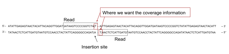Open image in new tab

Hands-on: Compute genome coverage

1. bamCoverage tool with:
   • param-collection “BAM/CRAM file”: collection output of the last Map with Bowtie for Illumina
   • “Bin size in bases”: 1
   • “Scaling/Normalization method”: Do not normalize or scale
   • “Coverage file format”: bedgraph
   • “Show advanced options”: yes
     • “Ignore missing data?”: Yes (to get only region with read counts)
     • “Offset inside each alignment to use for the signal location”: -1 (to read the signal of the coverage only at the 3’ end of the read)

Identify TA sites positions

In order to get the coverage on each TA site we need to prepare a file containing the position of each TA site.

As you can see on the previous figure, the read can cover one side or the other of the TA depending on the direction of insertion of the transposon. Depending on the direction of insertion the coverage will be counted on the leftmost position of the TA site or on the rightmost. As we are not considering strand separately in this analyses, we will consider both count as attached to the leftmost base of the TA site. To do that we will create two list of TA site positions, listing the 5’ end of each TA site for forward and reverse strand, and then merge them to get a global count per TA site.

Hands-on: Get TA sites coordinates

1. Nucleotide subsequence search tool with:
   • param-file Nucleotide sequence to be searched”: staph_aur.fasta
   • “Search with a”: user defined pattern
   • “Search pattern”: TA
   • “Search pattern on”: forward strand
2. Inspect the generated file

Nucleotide subsequence search generate one BED file with the coordinates of each TA on the genome:

1. Chrom
2. Start
3. End
4. Name
5. Strand

The only information we need here are the positions of the 5’ end of each TA site for each strand.

Hands-on: Get forward and reverse strand positions

1. Cut columns from a table tool with:
   • Cut columns : c2
   • “Delimited by”: tab
   • param-file “From”: output of Nucleotide subsequence search

2. Add the #forward tag to the output

   Tip: Adding a tag

   Datasets can be tagged. This simplifies the tracking of datasets across the Galaxy interface. Tags can contain any combination of letters or numbers but cannot contain spaces.

   To tag a dataset:

   1. Click on the dataset to expand it
   2. Click on Add Tags galaxy-tags
   3. Add tag text. Tags starting with # will be automatically propagated to the outputs of tools using this dataset (see below).
   4. Press Enter
   5. Check that the tag appears below the dataset name

   Tags beginning with # are special!

   They are called Name tags. The unique feature of these tags is that they propagate: if a dataset is labelled with a name tag, all derivatives (children) of this dataset will automatically inherit this tag (see below). The figure below explains why this is so useful. Consider the following analysis (numbers in parenthesis correspond to dataset numbers in the figure below):

   1. a set of forward and reverse reads (datasets 1 and 2) is mapped against a reference using Bowtie2 generating dataset 3;
   2. dataset 3 is used to calculate read coverage using BedTools Genome Coverage separately for + and - strands. This generates two datasets (4 and 5 for plus and minus, respectively);
   3. datasets 4 and 5 are used as inputs to Macs2 broadCall datasets generating datasets 6 and 8;
   4. datasets 6 and 8 are intersected with coordinates of genes (dataset 9) using BedTools Intersect generating datasets 10 and 11.

   

   Now consider that this analysis is done without name tags. This is shown on the left side of the figure. It is hard to trace which datasets contain “plus” data versus “minus” data. For example, does dataset 10 contain “plus” data or “minus” data? Probably “minus” but are you sure? In the case of a small history like the one shown here, it is possible to trace this manually but as the size of a history grows it will become very challenging.

   The right side of the figure shows exactly the same analysis, but using name tags. When the analysis was conducted datasets 4 and 5 were tagged with #plus and #minus, respectively. When they were used as inputs to Macs2 resulting datasets 6 and 8 automatically inherited them and so on… As a result it is straightforward to trace both branches (plus and minus) of this analysis.

   More information is in a dedicated #nametag tutorial.

3. Cut columns from a table tool with:
   • Cut columns : c1,c3
   • “Delimited by”: tab
   • param-file “From”: output of Nucleotide subsequence search
4. Compute an expression on every row tool to shift the end position of TA sites by 1 and get the start of the TA site on the reverse strand with:
   • Add expression”: c2-1
   • param-file “as a new column to”: output of cut
   • “Round result?”: yes
5. Cut columns from a table tool with:
   • Cut columns : c3
   • “Delimited by”: tab
   • param-file “From”: output of Compute
6. Add the #reverse tag to the output

Merge overall coverage and positions of TA sites to get the coverage of each TA sites

We have now 2 files containing the coordinates of our TA sites for both strands. We should cross them with the coverage files to get the coverage on both sides of each TA site.

Hands-on: Get coverage of TA sites

1. Join two files tool with:
   • param-collection 1st file”: output of bamCoverage
   • “Column to use from 1st file”: Column 2 (to select the position of the end of the read)
   • param-file “2nd File”: output of last cut with the forward tags
   • “Column to use from 2nd file”: Column 1
   • “Output lines appearing in”: Both 1st & 2nd file, plus unpairable lines from 2st file. (-a 2) (to get all TA sites)
   • “First line is a header line”: No
   • “Value to put in unpaired (empty) fields”: 0 (to assign a count of 0 to TA sites not covered in the bamCoverage file)

2. Add #forward tag to the output collections

   Tip: Adding a tag to a collection

   1. Click on the collection in your history to view it
   2. Click on Edit galaxy-pencil next to the collection name at the top of the history panel
   3. Click on Add Tags galaxy-tags
   4. Add a tag starting with #
      • Tags starting with # will be automatically propagated to the outputs any tools using this dataset.
   5. Click Save galaxy-save
   6. Check that the tag appears below the collection name

3. Cut columns from a table tool with:
   • Cut columns : c1,c4
   • “Delimited by”: tab
   • param-file “From”: output ofJoin two files with the forward tag
4. Repeat the same steps for reverse

We now have a read count for each nucleotide at the different TA sites. The insertions on the forward strand files are in a different direction than those on the reverse strand file. In our case, we are only interested in studying the gene disruption, and therefore we do not want to consider the directions separately. We can then combine the forward and reverse counts together to get a total count per TA site. In order to do that we need to assign the count of both strand to the same nucleotide, by shifting by one position the count on the reverse strand.

Hands-on: Get total count per TA site

1. Compute an expression on every row tool to shift the positions of reverse strand counts with:
   • Add expression”: c1-1 (to shift the position by 1)
   • param-collection “as a new column to”: Cut output collection with the tags reverse
   • “Round result?” : yes
2. Cut columns from a table tool with:
   • “Cut columns”: c3,c2
   • “Delimited by”: tab
   • param-collection File to cut”: output of the previous Compute
3. Sort tool with:
   • param-collection “Sort Query”: the newest reverse collection
   • “Number of header lines”: 0
   • In “Column selections”
     • “on column”: Column: 1 (to sort on positions)
     • “in”: Ascending Order
     • “Flavor”: Fast numeric sort (-n)

4. Repeat the Sort with the newest forward collection

5. Join two files tool to merge the two collections and get the forward and reverse count in two different columns with:
   • param-collection 1st file” : the forward collection from Sort
   • “Column to use from 1st file”: Column 1 to join on positions
   • param-collection “2nd File” : the reverse collection from Sort
   • “Column to use from 2nd file”: Column 1
   • “Output lines appearing in”: Both 1st & 2nd file (to get all TA sites)
   • “First line is a header line”: No
   • “Value to put in unpaired (empty) fields”: .
6. Compute an expression on every row tool to get the total read count with:
   • Add expression”: c2+c3 to get the total count
   • param-collection “as a new column to”: output of Join two files with the tags reverse and forward
   • “Round result?”: yes
7. Cut columns from a table tool with:
   • “Cut columns”: c1,c4
   • “Delimited by”: tab
   • param-collection File to cut”:output of the last Compute
8. Sort data in ascending or descending order tool with:
   • param-collection Sort Query”: output of the last Cut
   • “Number of header lines”: 0
   • In “Column selections”
     • “on column”: Column: 1 (to sort on positions)
     • “in”: Ascending Order
     • “Flavor”: Fast numeric sort (-n)

Question

Take a look at the output files:

1. What are the data contained in the two columns?
2. What do the 5 first lines of the blunt sample in the treatment with the condition look like?

Solution

1. The first column contain the position of the TA site, and the second column the number of insertions observed.
2. Your five first lines should look like this :
   • One column with the positions : 4,10,16,42,79
   • One column with the number of insertions : 0,3,20,0,11

If your counts are only zeros in one of the blunt sample, you might have made a mistake in merging the counts to the TA sites.

Predicting Essential Genes with Transit

Now that we have the counts of insertions per TA site, we can use them to predict gene essentiality. Several methods exist to identify essential genes of regions. They can be divided in two major categories:

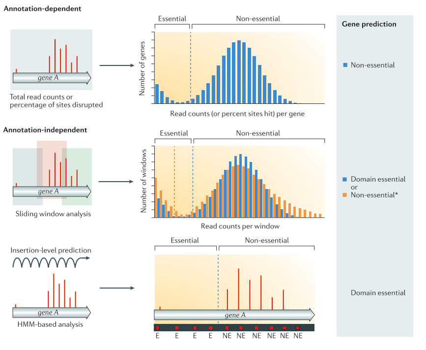Open image in new tab

1. Annotation dependent method

   The total read count an/or percentage of disrupted site are computed per annotated regions. The values are then compared to the rest of the genome to classify the genes into the categories essential or non-essential.

2. Annotation independent method

   The total read count and/or disrupted sites are computed independently of annotated regions. One of these methods is using a sliding window. Each window is then classified into the categories essential or non-essential. After the windows have been classified, they are linked annotations, and the genes/regions can be classified as essential, non-essential, or domain essential according to the classification of the windows they cover. The same classification can be done using HMM based methods instead of sliding windows. In that case, each insertion site will be predicted as essential or non essential Chao et al. 2016).

To predict the essential genes in our datasets, we will use the Transit tool DeJesus et al. 2015.

Transit

Transit is a software that can be used to analyse TnSeq Data. It is compatible with Mariner and Tn5 transposon. In total, 3 methods are available to assess gene essentiality in one sample.

Gumbel method

The Gumbel method performs a gene by gene analysis of essentiality for Mariner data based on the longest consecutive sequence of TA site without insertions in a gene. This allows to identify essential domains regardless of insertion at other location of the gene.

The distribution governing the longest sequence of consecutive non insertion is characterized by a Gumbel distribution. This distribution is often used to model the distribution of maximums (or minimums) of a variable (See the Wikipedia article on Gumbel distribution ). The Gumbel distribution is used as a likelihood of non-essentiality, as the longest run of non-insertions should follow what is expected given the global distribution of non-insertion runs. The essential genes, whose runs of empty sites are longer than expected, are modeled through a normalized sigmoid function. This function reflect that any gene can be essential, except the gene were the run of non insertions are too smell to represent a domain.

The total distribution of the maximum run of non-insertion per gene is therefore represented y a bimodal distribution composed of a Gumbel distribution of non-essential genes and a normalized sigmoid function of essential ones. The parameters of these distributions are estimated through a Metropolis–Hastings (MH) sampling procedure DeJesus et al. 2013).

Using these two distribution, the posterior probability of each distribution is calculated for each gene. Some genes can be classified as “Unclear” if one probability is not winning over the other. Some other can be classified as “Small” if the space of TA sites covered by the gene is insufficient to categorize it (See the Transit Manual for the Gumbel method).

HMM method

The HMM method performs a whole genome essentiality analysis for Mariner data. This approach uses the clustering of TA sites along the genome to identify essential regions, and then apply results to the annotation to identify genes containing essential regions. The HMM method provides a classification for each TA site into 4 states : Essential, Non-Essential, Growth Advantage, and Growth Defect.

This method require a well-saturated library and is sensitive to sparse datasets DeJesus and Ioerger 2013.

Tn5Gaps method

The Tn5Gaps method is a method dedicated to the identification of essential genes in studies using Tn5 transposons. The analysis is performed on the whole genome to identify regions of non insertion overlapping with genes. It is based on a Gumbel analysis method Griffin et al. 2011 and adapted to Tn5 transposon specificity. The main difference comes from the fact that Tn5 transposon can insert everywhere, thus creating libraries with lower insertion rates. The difference from the Gumbel method described above is that the run of non insertion are computer on the whole genome instead of individual genes. The longest run of non insertion considered is not the longest within the gene, but the longest one overlapping the gene.

Predict the essentiality of genes

In our case, we will use the Gumbel method, because we are using Mariner data and our data look pretty sparse. Gumbel is therefore the safe choice compared to HMM which is more sensitive to sparse data.

In order to use transit, we need to create a an annotation file in the prot_table format, specific to the Transit tool. It can be created this file from a GFF3 from GenBank like the one we uploaded earlier.

Hands-on: Hands-on : Create annotation file in prot_table format

1. Check that the format of staph_aur.gff3 file is gff3 and not gff

2. Change the datatype if needed

   Tip: Changing the datatype

   • Click on the galaxy-pencil pencil icon for the dataset to edit its attributes
   • In the central panel, click galaxy-chart-select-data Datatypes tab on the top
   • In the galaxy-chart-select-data Assign Datatype, select gff3 from “New type” dropdown
     • Tip: you can start typing the datatype into the field to filter the dropdown menu
   • Click the Save button

3. Convert GFF3 to prot_table for TRANSIT tool with:
   • param-file GenBank GFF file”: the staph_aur.gff3 file

Now that we have prepared the annotation file, we can use the count per TA site to predict essential genes using Transit tool, with some customized parameters:

• The number of sites with a single read could be artefactual. We ignore then counts lower than 2
• A disrupted site that would be very close to the border of the gene may not actually disturb the gene function, and therefore not be an actual signal of disruption. We ignore then insertion near the extremities of the genes.

Hands-on: Predict gene essentiality with Transit

1. Gumbel tool with:
   • “Operation mode”: Replicates
     • param-collection “Input .wig files”: output of the latest Sort
   • param-file “Input annotation”: output of the latest Convert
   • “Smallest read-count to consider”: 2 (to ignore single count insertions)
   • “Ignore TAs occurring at given fraction of the N terminus.”: 0.1 (to ignore 10% of the insertion at the N-terminus extremity of the gene)
   • “Ignore TAs occurring at given fraction of the C terminus.”: 0.1 (to ignore 10% of the insertion at the C-terminus extremity of the gene)

The output of Transit is a tabulated file containing the following columns:

• Gene ID
• Name of the gene
• Gene description
• Number of Transposon Insertions Observed within the Gene
• Total Number of TA sites within the Gene
• Length of the Maximum Run of Non-Insertions observed (in number of TA sites)
• Span of nucleotides for the Maximum Run of Non-Insertions
• Posterior Probability of Essentiality
• Essentiality call for the gene
  • E=Essential
  • U=Uncertain
  • NE=Non-Essential
  • S=too short

Comment: More details about Transit

You can find more information on Transit manual page

We can obtain the list of genes predicted as essential by filtering on the essentiality call.

Hands-on: Hands-on : Get table of essential genes

1. Filter data on any column using simple expressions tool with:
   • param-collection “Filter”: output of the last Gumbel
   • With following condition”: c9=='E' (to select essential genes)

Question

How many genes are essential in each conditions?

Solution

359 genes are essential in control, and 381 in condition.

Compare the essential genes between two conditions

Now let’s compare the results between out two conditions.

Hands-on: Separate Files from the collection

1. Extract Dataset from a list tool to extract 1st file in the collection with:
   • param-collection Input List”: output of the last Filter
   • How should a dataset be selected?”: Select by index
     • Element index:”: 0 to select the first dataset

2. Add the #condition tag

3. Extract Dataset from a list tool to extract 2nd file in the collection with:
   • param-collection Input List”: output of the last Filter
   • How should a dataset be selected?”: Select by index
     • Element index:”: 1 to select the second dataset
4. Add the #control tag

We would like now to get the list of essential gene in both conditions

Hands-on: Get gene essential in both conditions

1. Join two files tool with:
   • param-file 1st file”: output of Extract Dataset with control tag
   • Column to use from 1st file”: Column : 1 (to compare on gene ID)
   • param-file 2nd file”: output of Extract Dataset with condition tag
   • Column to use from 2nd file”: Column : 1 (to compare on gene ID)
   • Output lines appearing in”: Both 1st and 2nd files (to get common essential genes)

Let’s now get the list of essential gene that are different between the two conditions.

Hands-on: Get gene essential only in control

1. Join two files tool with:
   • param-file 1st file”: output of Extract Dataset with control tag
   • Column to use from 1st file”: Column : 1 (to compare on gene ID)
   • param-file 2nd file”: output of Extract Dataset with condition tag
   • Column to use from 2nd file”: Column : 1 (to compare on gene ID)
   • Output lines appearing in”: 1st but not 2nd

Hands-on: Hands-on : Get gene essential only in condition

1. Join two files tool with:
   • 1st file”: output of Extract Dataset with control tag
   • Column to use from 1st file”: Column : 1 (to compare on gene ID)
   • 2nd file”: output of Extract Dataset with condition tag
   • Column to use from 2nd file”: Column : 1 (to compare on gene ID)
   • Output lines appearing in”: 2nd but not 1st

Question

1. How many genes are essential in both conditions?
2. How many genes are essential only in control?
3. How many genes are essential only in condition?

Solution

1. 320 genes are essential in both conditions.
2. 39 genes are essential only in control.
3. 61 genes are essential only in condition.

Conclusion

In this tutorial, we learned how to predict essential genes in different conditions. Although it seems to be a long process, keep in mind that the steps allowing to get the list of TA site does not need to be repeated for each analysis as long as you study the same genome. For repetitive analyses, the steps are fewer : mapping, coverage, attribution to TA sites, merging of strands and Transit analysis.

This tutorial focused on simple gene essentiality prediction in individual samples. You could be interested in intergenic regions as well, or comparing many samples together. Other methods exist in transit for these goals, that follow the same workflow. It is important to look at your data and to perform quality control to evaluate the coverage and sparsity of your data. This will influence not only the choice of method (HMM does not manage sparse data well), but the choice of parameters for your analysis.

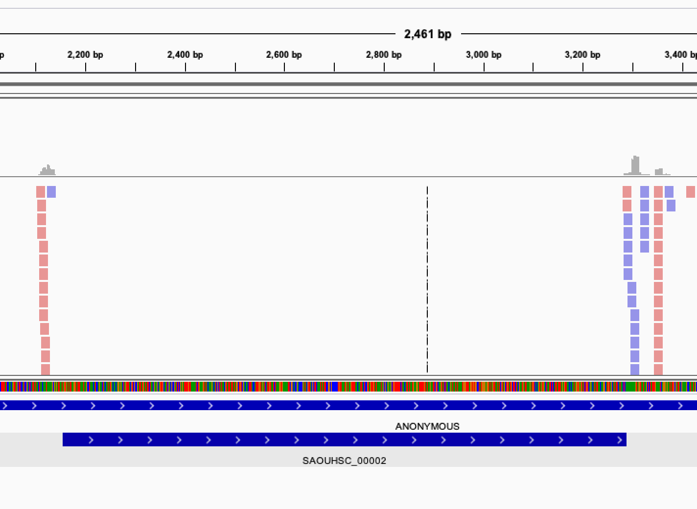
Once you get this list of gene, it is interesting to verify manually the genes classified as essentials. In order to do that, you can visualize the read mapped on your genome by displaying the bam files in IGV.

Tip: Add genome and annotations to IGV from Galaxy

1. Upload a FASTA file with the reference genome and a GFF3 file with its annotation in the history (if not already there)
2. Install IGV (if not already installed)
3. Launch IGV on your computer
4. Expand the FASTA dataset with the genome in the history
5. Click on the local in display with IGV to load the genome into the IGV browser
6. Wait until all Dataset status are ok

7. Close the window

   An alert ERROR Parameter "file" is required may appear. Ignore it.

8. Expand the GFF3 dataset with the annotations of the genome in the history
9. Click on the local in display with IGV to load the annotation into the IGV browser

10. Switch to the IGV instance

    The annotation track should appear. Be careful that all files have the same genome ID

Tip: Add Mapped reads track to IGV from Galaxy

1. Install IGV (if not already installed)
2. Launch IGV on your computer
3. Check if the reference genome is available on the IGV instance
4. Expand the BAM dataset with the mapped reads in the history
5. Click on the local in display with IGV to load the reads into the IGV browser

6. Switch to the IGV instance

   The mapped reads track should appear. Be sure that all files have the same genome ID

When looking at the read mapping at the location of predicted essential genes, you may encounter several situation: Some gene will have no read at all mapping to them, some will have an empty region, while other will have no clearly defined empty region but a very low count of reads, possibly indicating a growth defect induced by the gene disruption.

Open image in new tab

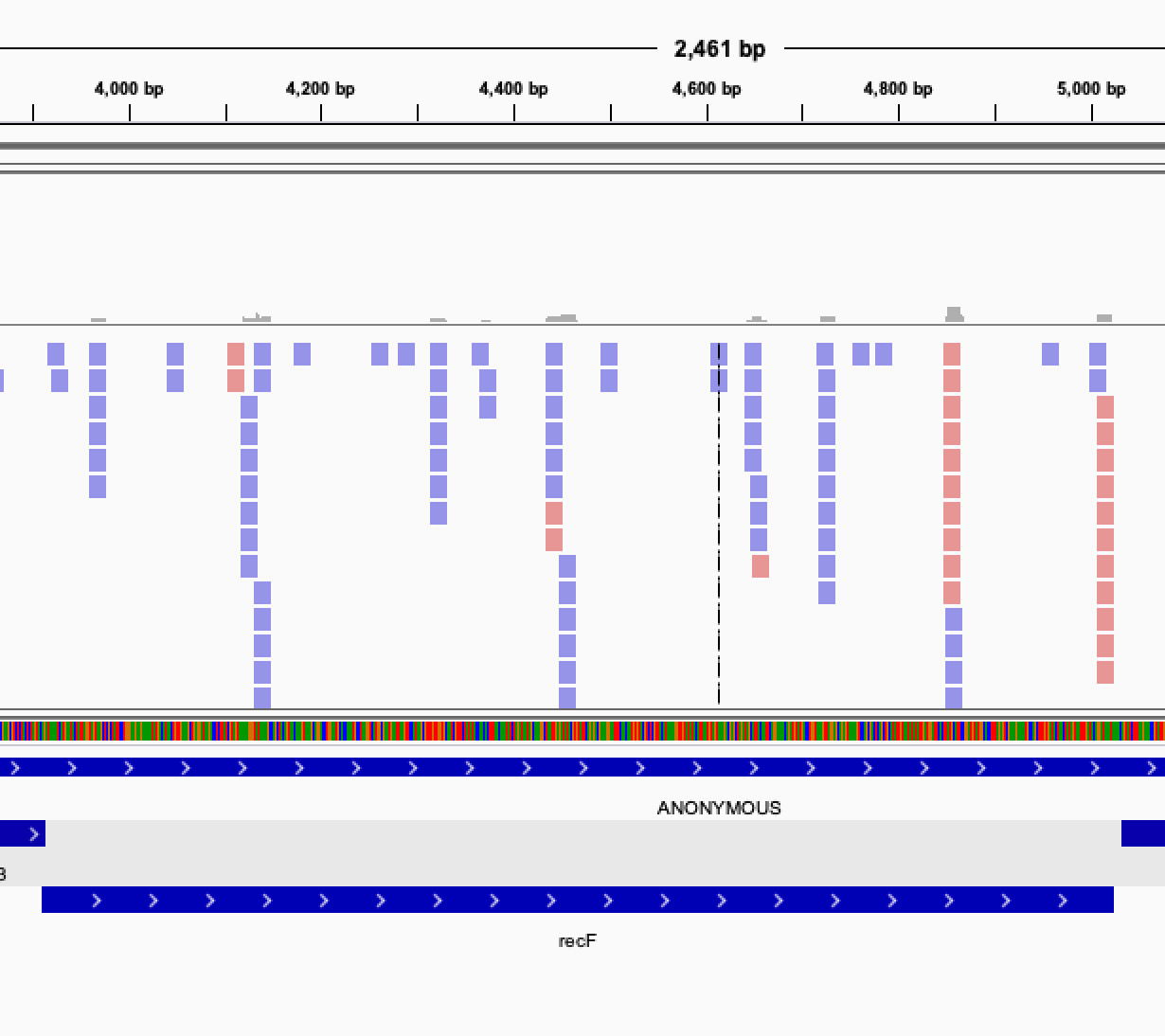Open image in new tab

Once you have curated and confirm the genes that appear essential, comparing the annotation of essential genes with the condition of growth will allow you a better understanding of certain mechanism of interest, like the gene involved in resistance to stress for example.

A comparison with published results of essentiality in your organism will be useful but don’t expect to find exactly the same results. The conditions of growth differ from one experiment to another, and can highly influence the detection of essential genes.

You've Finished the Tutorial

Please also consider filling out the Feedback Form as well!

Key points

• TnSeq is a useful analysis to detect essential genes and conditional essential genes

• The saturation of the library must be sufficient so that every gene must have been impacted at least once

• Be sure you have removed every transposon sequence before starting your analysis

• Verify the results manually do separate domain essential and essential genes

Frequently Asked Questions

References

1. Griffin, J. E., J. D. Gawronski, M. A. DeJesus, T. R. Ioerger, B. J. Akerley et al., 2011 High-resolution phenotypic profiling defines genes essential for mycobacterial growth and cholesterol catabolism. PLoS pathogens 7: e1002251. 10.1371/journal.ppat.1002251
2. DeJesus, M. A., and T. R. Ioerger, 2013 A hidden Markov model for identifying essential and growth-defect regions in bacterial genomes from transposon insertion sequencing data. BMC bioinformatics 14: 303. 10.1186/1471-2105-14-303
3. DeJesus, M. A., Y. J. Zhang, C. M. Sassetti, E. J. Rubin, J. C. Sacchettini et al., 2013 Bayesian analysis of gene essentiality based on sequencing of transposon insertion libraries. Bioinformatics 29: 695–703. 10.1093/bioinformatics/btt043
4. DeJesus, M. A., C. Ambadipudi, R. Baker, C. Sassetti, and T. R. Ioerger, 2015 TRANSIT-a software tool for Himar1 TnSeq analysis. PLoS computational biology 11: e1004401. 10.1371/journal.pcbi.1004401
5. Kwon, Y. M., S. C. Ricke, and R. K. Mandal, 2015 Transposon sequencing: methods and expanding applications. Applied Microbiology and Biotechnology 100: 31–43. 10.1007/s00253-015-7037-8
6. Santiago, M., L. M. Matano, S. H. Moussa, M. S. Gilmore, S. Walker et al., 2015 A new platform for ultra-high density Staphylococcus aureus transposon libraries. BMC Genomics 16: 10.1186/s12864-015-1361-3
7. Chao, M. C., S. Abel, B. M. Davis, and M. K. Waldor, 2016 The design and analysis of transposon insertion sequencing experiments. Nature Reviews Microbiology 14: 119–128. 10.1038/nrmicro.2015.7

Feedback

Did you use this material as an instructor? Feel free to give us feedback on how it went.
Did you use this material as a learner or student? Click the form below to leave feedback.

Citing this Tutorial

1. Delphine Lariviere, Bérénice Batut, Essential genes detection with Transposon insertion sequencing (Galaxy Training Materials). https://training.galaxyproject.org/training-material/topics/genome-annotation/tutorials/tnseq/tutorial.html Online; accessed TODAY
2. Hiltemann, Saskia, Rasche, Helena et al., 2023 Galaxy Training: A Powerful Framework for Teaching! PLOS Computational Biology 10.1371/journal.pcbi.1010752
3. Batut et al., 2018 Community-Driven Data Analysis Training for Biology Cell Systems 10.1016/j.cels.2018.05.012

BibTeX

@misc{genome-annotation-tnseq,
author = "Delphine Lariviere and Bérénice Batut",
	title = "Essential genes detection with Transposon insertion sequencing (Galaxy Training Materials)",
	year = "",
	month = "",
	day = "",
	url = "\url{https://training.galaxyproject.org/training-material/topics/genome-annotation/tutorials/tnseq/tutorial.html}",
	note = "[Online; accessed TODAY]"
}
@article{Hiltemann_2023,
	doi = {10.1371/journal.pcbi.1010752},
	url = {https://doi.org/10.1371%2Fjournal.pcbi.1010752},
	year = 2023,
	month = {jan},
	publisher = {Public Library of Science ({PLoS})},
	volume = {19},
	number = {1},
	pages = {e1010752},
	author = {Saskia Hiltemann and Helena Rasche and Simon Gladman and Hans-Rudolf Hotz and Delphine Larivi{\`{e}}re and Daniel Blankenberg and Pratik D. Jagtap and Thomas Wollmann and Anthony Bretaudeau and Nadia Gou{\'{e}} and Timothy J. Griffin and Coline Royaux and Yvan Le Bras and Subina Mehta and Anna Syme and Frederik Coppens and Bert Droesbeke and Nicola Soranzo and Wendi Bacon and Fotis Psomopoulos and Crist{\'{o}}bal Gallardo-Alba and John Davis and Melanie Christine Föll and Matthias Fahrner and Maria A. Doyle and Beatriz Serrano-Solano and Anne Claire Fouilloux and Peter van Heusden and Wolfgang Maier and Dave Clements and Florian Heyl and Björn Grüning and B{\'{e}}r{\'{e}}nice Batut and},
	editor = {Francis Ouellette},
	title = {Galaxy Training: A powerful framework for teaching!},
	journal = {PLoS Comput Biol}
}

                   

Galaxy Administrators: Install the missing tools

You can use Ephemeris's shed-tools install command to install the tools used in this tutorial.

shed-tools install [-g GALAXY] [-a API_KEY] -t <(curl https://training.galaxyproject.org/training-material/api/topics/genome-annotation/tutorials/tnseq/tutorial.json | jq .admin_install_yaml -r)

Alternatively you can copy and paste the following YAML

---
install_tool_dependencies: true
install_repository_dependencies: true
install_resolver_dependencies: true
tools:
- name: deeptools_bam_coverage
  owner: bgruening
  revisions: bb1e4f63e0e6
  tool_panel_section_label: deepTools
  tool_shed_url: https://toolshed.g2.bx.psu.edu/
- name: find_subsequences
  owner: bgruening
  revisions: d882a0a75759
  tool_panel_section_label: Annotation
  tool_shed_url: https://toolshed.g2.bx.psu.edu/
- name: text_processing
  owner: bgruening
  revisions: d698c222f354
  tool_panel_section_label: Text Manipulation
  tool_shed_url: https://toolshed.g2.bx.psu.edu/
- name: text_processing
  owner: bgruening
  revisions: d698c222f354
  tool_panel_section_label: Text Manipulation
  tool_shed_url: https://toolshed.g2.bx.psu.edu/
- name: bowtie_wrappers
  owner: devteam
  revisions: b46e7d48076a
  tool_panel_section_label: Mapping
  tool_shed_url: https://toolshed.g2.bx.psu.edu/
- name: column_maker
  owner: devteam
  revisions: be25c075ed54
  tool_panel_section_label: Text Manipulation
  tool_shed_url: https://toolshed.g2.bx.psu.edu/
- name: gff_to_prot
  owner: iuc
  revisions: 07d7991bf205
  tool_panel_section_label: Annotation
  tool_shed_url: https://toolshed.g2.bx.psu.edu/
- name: transit_gumbel
  owner: iuc
  revisions: f50807720df1
  tool_panel_section_label: Annotation
  tool_shed_url: https://toolshed.g2.bx.psu.edu/
- name: cutadapt
  owner: lparsons
  revisions: 49370cb85f0f
  tool_panel_section_label: FASTA/FASTQ
  tool_shed_url: https://toolshed.g2.bx.psu.edu/

Feedback

5 stars	3
3 stars	1

August 2022

• 5 stars: Liked: everything.. thanks for this Disliked: i cant find bowtie tools.. only bowtie 2, but the parameters described here are for bowtie.

August 2021

• 5 stars: Liked: very clear Disliked: r code