The Vertebrate Genome Project (VGP), a project of the Genome 10K (G10K) Consortium, aims to generate high-quality, near error-free, gap-free, chromosome-level, haplotype-phased, annotated reference genome assemblies for every vertebrate species (Rhie et al. 2020). The VGP has developed a fully automated de-novo genome assembly pipeline, which uses a combination of three different technologies: Pacbio high fidelity reads (HiFi), all-versus-all chromatin conformation capture (Hi-C) data, and (optionally) Bionano optical map data. The pipeline consists of nine distinct workflows. This tutorial provides a quick example of how to run these workflows for one particular scenario, which is, based on our experience, the most common: assembling genomes using HiFi Reads combined with Hi-C data (both generated from the same individual).
This tutorial assumes you are comfortable getting data into Galaxy, running jobs, managing history, etc. If you are unfamiliar with Galaxy, we recommend you visit the Galaxy Training Network. Consider starting with the following trainings:
Better haplotype resolution and improved continuity
F
HiFi + parental + Bionano
Better haplotype resolution and improved continuity
G
HiFi + parental data + Hi-C + Bionano
Better haplotype resolution and ultimate continuity
H
In this table, HiFi and Hi-C data are derived from the individual whose genome is being assembled. “Parental data” refers to high coverage whole genome resequencing data from the parents of the individual being assembled. Assemblies utilizing parental data for phasing are also called “Trios”. Each combination of input datasets is supported by an analysis trajectory: a combination of workflows designed for generating assembly given a particular combination of inputs. These trajectories are listed in the table above and shown in the figure below.
Figure 1: Eight analysis trajectories are possible depending on the combination of input data. A decision on whether or not to invoke Workflow 6 is based on the analysis of QC output of workflows 3, 4, or 5. Thicker lines connecting Workflows 7, 8, and 9 represent the fact that these workflows are invoked separately for each phased assembly (once for maternal and once for paternal).
The first stage of the pipeline is the generation of a k-mer profile of the raw reads to estimate genome size, heterozygosity, repetitiveness, and error rate necessary for parameterizing downstream workflows. The generation of k-mer counts can be done from HiFi data only (Workflow 1) or include data from parental reads for trio-based phasing (Workflow 2). The second stage is contig assembly. In addition to using only HiFi reads (Workflow 3), the contig-building (contiging) step can leverage Hi-C (Workflow 4) or parental read data (Workflow 5) to produce fully-phased haplotypes (hap1/hap2 or parental/maternal assigned haplotypes), using hifiasm. The contiging workflows also produce a number of critical quality control (QC) metrics such as k-mer multiplicity profiles. Inspection of these profiles provides information to decide whether the third stage—purging of false duplication—is required. Purging (Workflow 6), using purge_dups identifies and resolves haplotype-specific assembly segments incorrectly labeled as primary contigs, as well as heterozygous contig overlaps. This increases continuity and the quality of the final assembly. The purging stage is generally unnecessary for trio data, as thses assemblies achieve reliable haplotype resolution using k-mer set operations based on parental reads. Generally, HiC-phased contigs also do not need to undergo purging, but if so, then there exists Workflow 6b to purge a single haplotype at a time. The fourth stage, scaffolding, produces chromosome-level scaffolds using information provided by Bionano (Workflow 7), with Bionano Solve (optional) and Hi-C (Workflow 8) data and YaHS algorithms. A final stage of decontamination (Workflow 9) removes exogenous sequences (e.g., viral and bacterial sequences) from the scaffolded assembly. A separate workflow (WF0) is used to assemble and annotate a mitogenome.
Comment: A note on data quality
We suggest at least 30✕ PacBio HiFi coverage and 60✕ Hi-C coverage (both diploid coverage).
Getting the data
The following steps use PacBio HiFi and Illumina Hi-C data from baker’s yeast (Saccharomyces cerevisiae). The tutorial represents trajectory B from Fig. 1 above. For this tutorial, the first step is to get the datasets from Zenodo. Specifically, we will be uploading two datasets:
A set of PacBio HiFi reads in fasta format. Please note that your HiFi reads received from a sequencing center will usually be fastqsanger.gz format, but the dataset used in this tutorial has been converted to fasta for space..
A set of Illumina Hi-C reads in fastqsanger.gz format.
Uploading fasta datasets from Zenodo
The following two steps demonstrate how to upload three PacBio HiFi datasets into your Galaxy history.
Hands On: Uploading FASTA datasets from Zenodo
Create a new history for this tutorial
To create a new history simply click the new-history icon at the top of the history panel:
Copy the following URLs into clipboard.
(You can do this by clicking on copy button in the right upper corner of the box below. It will appear if you mouse over the box.)
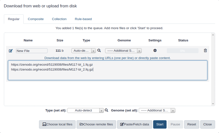
Click galaxy-uploadUpload at the top of the activity panel
Select galaxy-wf-editPaste/Fetch Data
Paste the link(s) into the text field
Change Type (set all): from “Auto-detect” to fasta
Press Start
Close the window
Uploading fastqsanger or fastqsanger.gz datasets via URL.
Click on Upload Data on the top of the left panel:
Click on Paste/Fetch:
Paste URL into text box that would appear:
Set Type (set all) to fastqsanger or, if your data is compressed as in URLs above (they have .gz extensions), to fastqsanger.gz
:
Warning: Danger: Make sure you choose corect format!
When selecting datatype in “Type (set all)” dropdown, make sure you select fastaqsanger or fastqsanger.gz BUT NOT fastqcssanger or anything else!
Warning: These datasets are large!
Hi-C datasets are large. It will take some time (~15 min) for them to be fully uploaded. Please, be patient.
Organizing the data
If everything goes smoothly, your history will look like shown in Fig. 4 below. The three HiFi fasta files and the two Hi-C files are better represented as collections: Galaxy’s way to represent multiple datasets as a single interface entity (collection). Paired data such as Hi-C reads are represented by a specific type of collection called paired collection: {paired-collection}
Also, importantly, the workflows we will be using for the analysis of our data takes collections as inputs (they do not access individual datasets). So let’s create collections using steps outlines in the Tips tip that you can find below Fig. 4.
Figure 2: History after uploading HiFi and Hi-C data (left). The creation of lists (collections) combines datasets into two items called 'HiFi data' and 'Hi-C data'(right). See below for instruction on how to make these collections.
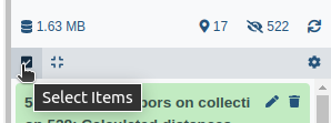
Click on galaxy-selectorSelect Items at the top of the history panel
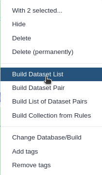
Check all the datasets in your history you would like to include
Click 3 of N selected and choose Advanced Build List
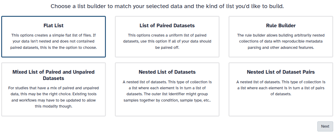
You are in collection building wizard. Choose Flat List and click ‘Next’ button at the right bottom corner.
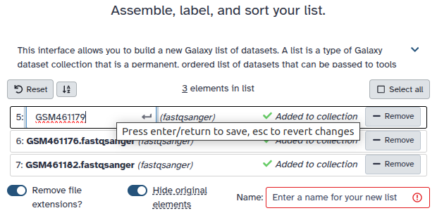
Double clcik on the file names to edit. For example, remove file extensions or common prefix/suffixes to cleanup the names.
Enter a name for your collection
Click Build to build your collection
Click on the checkmark icon at the top of your history again
Click on galaxy-selectorSelect Items at the top of the history panel
Check all the datasets in your history you would like to include
Click 2 of N selected and choose Advanced Build List
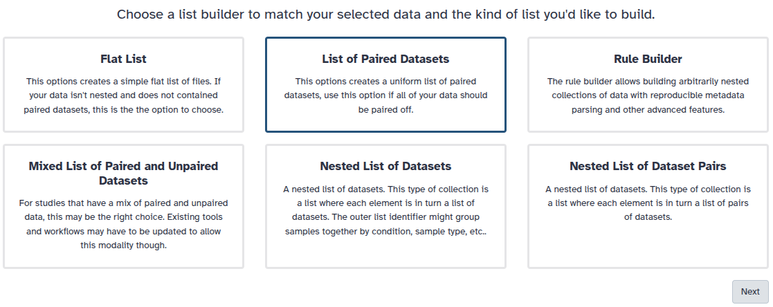
You are in the collection building wizard. Choose List of Paired Datasets and click ‘Next’ button at the right bottom corner.
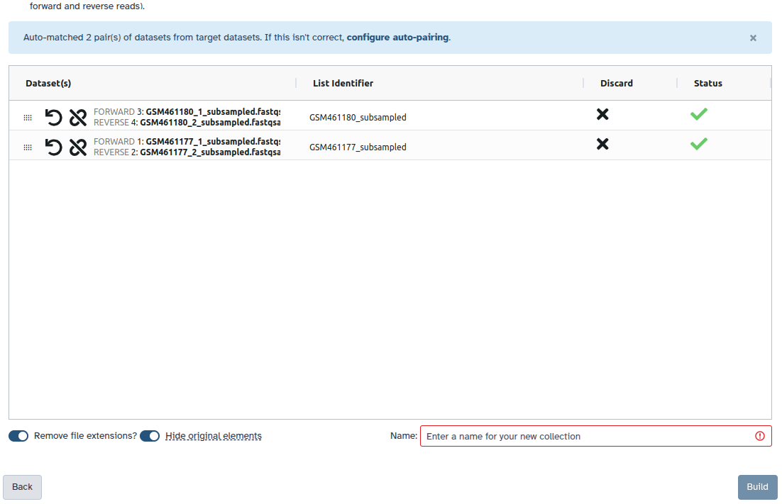
Check and configure auto-pairing. Commonly matepairs have suffix _1 and _2 or _R1 and _R2. Click on ‘Next’ at the bottom.
Edit the List Identifier as required.
Enter a name for your collection
Click Build to build your collection
Click on the checkmark icon at the top of your history again
You can obviously upload your own datasets via URLs as illustrated above or from your own computer. In addition, you can upload data from a major repository called GenomeArk. GenomeArk is integrated directly into Galaxy Upload. To use GenomeArk following the steps in the Tip tip below:
Open the file galaxy-uploadupload menu
Click on Choose remote files tab
Click on the Genome Ark button and then click on species
You can find the data by following this path: /species/${Genus}_${species}/${specimen_code}/genomic_data. Inside a given datatype directory (e.g.pacbio), select all the relevant files individually until all the desired files are highlighted and click the Ok button. Note that there may be multiple pages of files listed. Also note that you may not want every file listed.
Once we have imported the datasets, the next step is to import the workflows necessary for the analysis of our data from DockStore.
Importing workflows
All analyses described in this tutorial are performed using workflows–chains of tools–shown in Fig. 1. Specifically, we will use four workflows corresponding to analysis trajectory B: 1, 4, 6, and 8. To use these four workflows you need to import them into your Galaxy account following the steps below. Note: these are not necessarily the latest versions of the actual workflows, but versions that have been tested for this tutorial. To see the latest versions, see the IWC VGP workflows page and click on the workflows for details and links to import them. Alternatively, for each section of the tutorial, there will be a “Launch [workflow] (View on Dockstore)” link at the beginning, which you can use to launch the workflow.
Performing the assembly
Workflows listed in Fig. 1 support a variety of “analysis trajectories”. The majority of species that were sequenced by the VGP usually contain HiFi reads for the individual being sequenced supplemented with Hi-C data. As a result most assemblies performed by us follow the trajectory B. This is why this tutorial was designed to follow this trajectory as well.
Genome profile analysis (WF1)
Before the assembly can be run, we need to collect metrics on the properties of the genome under consideration, such as the expected genome size according to our data. The present pipeline uses Meryl for generating the k-mer database and Genomescope2 for determining genome characteristics based on a k-mer analysis.
Launching the workflow
Hands On: Importing and Launching a Dockstore Workflow
Figure 3: Workflow main menu. The workflow menu lists all the workflows that have been imported. It provides useful information for organizing the workflows, such as last update and the tags. The worklows can be run by clicking in the play icon, marked in red in the image.
Comment: K-mer length
In this tutorial, we are using a k-mer length of 31. This can vary, but the VGP pipeline tends to use a k-mer length of 21, which tends to work well for most mammalian-size genomes. There is more discussion about k-mer length trade-offs in the extended VGP pipeline tutorial.
Refill your coffee
Assembly is not exactly an instantaneous type of analysis - this workflow will take approximately 15 minutes to complete. The same is true for all the analyses in this tutorial.
Interpreting the results
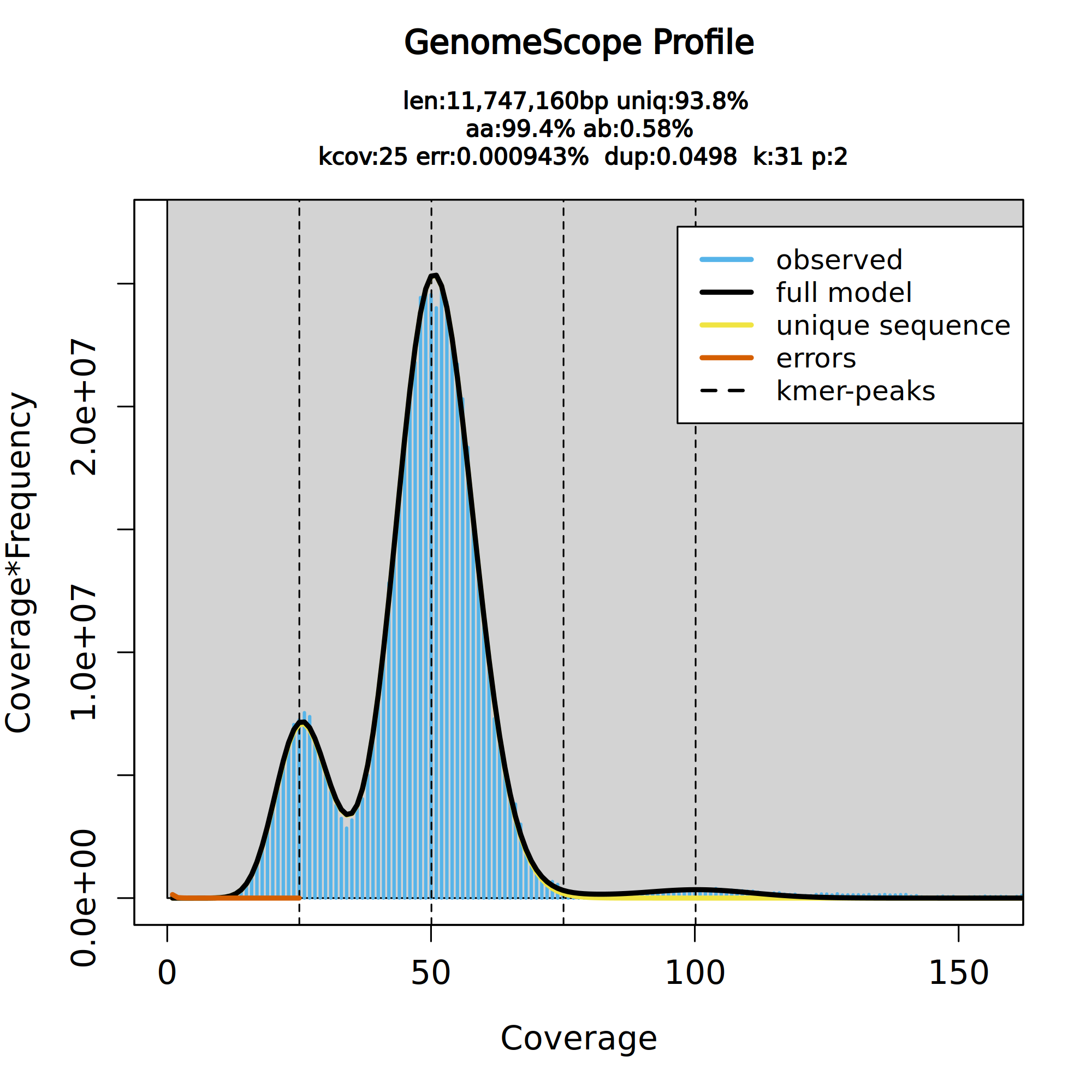
Once the workflow has finished, we can evaluate the transformed linear plot generated by Genomescope, which includes valuable information such as the observed k-mer profile, fitted models, and estimated parameters. This file corresponds to the dataset 18 in this history.
Figure 4: GenomeScope2 k-mer profile. The first peak located at about 25× corresponds to the heterozygous peak. The second peak at 50× corresponds to the homozygous peak. The plot also includes information about the inferred total genome length (len), genome unique length percent (uniq), overall heterozygosity rate (ab), mean k-mer coverage for heterozygous bases (kcov), read error rate (err), average rate of read duplications (dup) and k-mer size (k).
This distribution is the result of the Poisson process underlying the generation of sequencing reads. As we can see, the k-mer profile follows a bimodal distribution, indicative of a diploid genome. The distribution is consistent with the theoretical diploid model (model fit > 93%). Low frequency k-mers are the result of sequencing errors, and are indicated by the red line. Genomescope2 estimated a haploid genome size of around 11.7 Mbp, a value reasonably close to the Saccharomyces genome size. We are using the transformed linear plot because it shows the ploidy better by reducing low ccoverage peaks (like k-mers containing errors) and increasing higher coverage peaks (Ranallo-Benavidez et al. 2020).
It is worth noting that the genome characteristics such as length, error percentage, etc., are based on the GenomeScope2 model, which is the black line in the plot. If the model (black line) does not fit your observed data (blue bars), then these estimated characteristics might be very off. In the case of this tutorial, the model is a good fit to our data, so we can trust the estimates.
The workflow also generate a variety of quality control for your reads:
A heatmap generated by Mash Dist. This map shows the distance between your samples. This is a sanity check to verify all the read files belong to the same species. The tool developers(Ondov et al. 2016) identified the following distance breaks:
Same Species: <0.05
Same Genus: 0.05 to 0.34
Different Genus: >0.34
A Rdeval report including statistics on reads, such as length, quality and base composition.
Question: Heatmap
Look at the heatmap output. What is the highest Mash distance between our read libraries?
Figure 5: Mash Dist Heatmap. Each square is colored according to the distance between two set of reads. The diagonal is brown since the distance of one set with itself is 0. The closets sets are `01` and `03` in light blue (distance ~0.03), and `02` is a bit more distant with a distance of ~0.04 (dark teal)
The highest Mash distance between our read libraries is about 0.04 (see color scale legend).
Our libraries belong to the same species, since the threshold is 0.05.
Assembly (contiging) with hifiasm (WF4)
To generate contiguous sequences in an assembly (contigs) we will use the hifiasm assembler. It is a part of the “Assembly with HiC (WF4)” workflow . This workflow uses hifiasm (HiC mode) to generate HiC-phased haplotypes (hap1 and hap2). This is in contrast to its default mode, which generates primary and alternate pseudohaplotype assemblies. This workflow includes three tools for evaluating assembly quality: gfastats, BUSCO and Merqury.
Launching the workflow
Hands On: Importing and Launching a Dockstore Workflow
Click on “Galaxy” dropdown within the “Launch with” panel located in the upper right corner.
Select a galaxy instance you want to launch this workflow with.
You will be redirected to Galaxy and presented with a list of workflow versions.
Click the version you want (usually the latest labelled as “main”)
You are done!
The following short video walks you through this uncomplicated procedure:
Video: Importing from Dockstore
Hands On: Launching assembly (contiging) workflow
Identify inputs
The assembly workflow takes the following inputs:
HiFi reads as a collection
Whether we want to trim the Hi-C reads or not (Sometimes necessary with Arima Hi-C)
Hi-C reads as a paired collection
Genomescope Summary generated by previous (k-mer profiling) workflow
Meryl k-mer database generated by previous (k-mer profiling) workflow
Busco Database
Busco lineage
Name for Haplotype 1 (Used to generate QC files)
Name for Haplotype 2
Bits for bloom filter: Parameter impacting memory usage. Modify for large genomes.
Homozygous Read Coverage. Optional: set if you are unsatisfied with the Genomescope model.
Genomescope Model Parameters generated by previous (k-mer profiling) workflow
Launch the workflow
Click on the Workflow menu, located in the top bar
Click on the workflow-runRun workflow button corresponding to Assembly-Hifi-HiC-phasing-VGP4
In the Workflow: Assembly-Hifi-HiC-phasing-VGP4 menu fill the following parameters:
Species Name: Saccharomyces_cerevisiae
Assembly Name: gta26
param-collection “Pacbio Reads”: HiFi data collection
param-file “Hi-C reads”: Hi-C data
param-file “GenomeScope Summary”: GenomeScope on data X Summary (contains tag “GenomeScopeSummary”)
param-file “Meryl database”: Meryl on data X: read-db.mertyldb: the Meryl k-mer database (contains tag “MerylDatabase”)
“Database for Busco Lineage”: Busco v5 Lineage Datasets (or the latest version available in the instance)
“Provide lineage for BUSCO (e.g., Vertebrata)”: Ascomycota
param-file “GenomeScope Model Parameters”: GenomeScope on data X Model parameters (contains tag “GenomeScopeParameters”)
Click on the workflow-runRun workflow button
Comment: A note about "Homozygous Read Coverage"
Hifiasm tries to estimate the homozygous read coverage, but sometimes it can mistake a different peak as the homozygous coverage peak. To get around this, the VGP workflows calculate the homozygous coverage from the haploid coverage estimate from the GenomeScope outputs generated in the k-mer profiling workflow. However, sometimes GenomeScope can also misidentify the haploid peak, leading to it feeding an incorrect homozygous read coverage value into hifiasm. If this is the case, you can run the hifiasm workflows but specify the homozygous read coverage yourself. Otherwise, this parameter is fine to leave blank to let the workflows try to get it right on their own.
Interpreting the results
Warning: There will be two assemblies!
Because we are running hifiasm in HiC-phasing mode, it will produce two assemblies: hap1 and hap2!
Let’s have a look at the stats generated by gfastats. This output summarizes some main assembly statistics, such as contig number, N50, assembly length, etc. The workflow provide a joined table to display the statistics for both haplotype assemblies side-by-side. Below we provide a partial output of this file called Assembly statistics for Hap1 and Hap2 in your history:
Statistic
Hap 1
Hap 2
# contigs
16
17
Total contig length
11,304,582
12,160,988
Average contig length
706,536.38
715,352.24
Contig N50
922,430
923,452
Contig auN
895,015.76
904,515.33
Contig L50
5
6
Contig NG50
813,311
923,452
Contig auNG
861,281.68
936,364.22
Contig LG50
6
6
Largest contig
1,532,843
1,531,728
Smallest contig
185,224
85,850
According to the report, both assemblies are quite similar; the hap1 assembly includes 16 contigs, whose cumulative length is around 11.3 Mbp. The hap2 assembly includes 17 contigs, whose total length is 12.1Mbp. Both assemblies come close to the estimated genome size, which is as expected since we used hifiasm-HiC mode to generate phased assemblies, and this lowers the chance of false duplications that can inflate assembly size.
Comment: Are you working with pri/alt assemblies?
This tutorial uses the hifiasm-HiC workflow, which generates phased hap1 and hap2 assemblies. The phasing helps lower the chance of false duplications, since the phasing information helps the assembler know which genomic variation is heterozygosity at the same locus versus being two different loci entirely. If you are working with primary/alternate assemblies (especially if there is no internal purging in the initial assembly), you can expect higher false duplication rates than we observe here with the yeast HiC hap1/hap2.
Question
What is the longest contig in the hap1 assembly? And in the hap2 one?
What is the N50 of the hap2 assembly?
The longest contig in the hap1 assembly is 1,532,843 bp, and 1,531,728 bp in the hap2 assembly.
The N50 of the hap2 assembly is 923,452 bp.
Next, we are going to evaluate the outputs generated by Compleasm. This tool uses BUSCO to provides qualitative assessment of the completeness of a genome assembly in terms of expected gene content. It relies on the analysis of genes that should be present only once in a complete assembly or gene set, while allowing for rare gene duplications or losses (Simão et al. 2015).
The results are classified into five categories: complete and single-copy (S), complete and duplicated(D), fragmented(F), incomplete(I) and missing(M).
Question
How many BUSCO complete genes have been identified in the hap1 assembly?
How many BUSCO genes are absent in the hap1 assembly?
According to the summary, our assembly contains 1,526 complete BUSCO genes – this includes ones that are single-copy (S:86.75%, 1480) and ones that are duplicated (D:2.70%, 46).
158 BUSCO genes are missing.
Despite BUSCO being robust for species that have been widely studied, it can be inaccurate when the newly assembled genome belongs to a taxonomic group that is not well represented in OrthoDB. Merqury provides a complementary approach for assessing assembly quality in a reference-free manner via k-mer copy number analysis. Specifically, it takes our hap1 as the first genome assembly, hap2 as the second genome assembly, and the merylDB generated previously from our sequencing reads for k-mer counts.
By default, Merqury generates three collections as output: stats (completeness stats), plots and assembly consensus quality (QV) stats. Let’s first have a look at the copy number (CN) spectrum plot, known as the spectra-cn plot. The spectra-cn plot looks at both of your assemblies (here, your two haplotypes) taken together (fig. 6a).
Figure 6: Merqury CN plot for yeast assemblies. The plot tracks the multiplicity of each k-mer found in the read set and colors it by the number of times it is found in a given assembly. Merqury connects the midpoint of each histogram bin with a line, giving the illusion of a smooth curve. a). K-mer distribution of both haplotypes. b). K-mer distribution of an individual haplotype (hap2).
Our haplotypes look clean! In the spectra-cn plot for both haplotypes, the peaks are where we should expect them. There is a peak of k-mers present at 1-copy (so, only in either hap1 or hap2) with k-mer multiplicity of ~25, corresponding to heterozygous coverage. These are our heterozygous alleles being represented only once in our diplolid assemblies, which matches with their haploid coverage. We also have a peak of 2-copy k-mers present at diploid coverage, around ~50. This looks good so far, but we should also look at k-mer multiplicity for each individual haplotype separately, not just combined as they were in the previous plot. Figure 6b shows that most of the k-mers in our assembly are 1-copy – we have one copy of all the homozygous regions (the ones with 50x coverage) and of about half the heterozygous regions (the ones with 25x coverage). At the 25x coverage point, there is a “read-only” peak, which is expected, as these are the alternative alleles for those heterozygous loci, and those k-mers are likely in the other assembly, since they were not missing from the overall spectra-cn plot.
Hi-C scaffolding (WF8)
In this final stage, we will run the Scaffolding HiC YAHS (WF8) workflow, which uses the fact that the contact frequency between a pair of loci strongly correlates with the one-dimensional distance between them (i.e., linear distance on a chromosome). This information allows YAHS – the main tool in this workflow – to generate scaffolds that are often chromosome-sized.
Launching Hi-C scaffolding workflow
Warning: The scaffolding workflow is run on ONE haplotype at a time.
Contiging (VGP4) works with both (hap1/hap2, primary/alternate) assemblies simultaneously. This is not the case for contiging – it has to be run independently for each haplotype assembly. In this example (below) we run contiging on the hap1 assembly only. You can run the same analysis on the second haplotype by replacing hap1 with hap2.
Hands On: Importing and Launching a Dockstore Workflow
“Restriction enzymes”: Dovetail Omni-C: enzyme-free prep For this tutorial, we’ll use the Omni-C option as it is the equivalent of not specifying any restriction enzyme cutsites, but for your own data you would want to select the appropriate option.
param-file “Estimated genome size - Parameter File”: Estimated genome size: An output of the contiging workflow (VGP4) with a tag estimated_genome_size.
Click on the workflow-runRun workflow button
Interpreting the results
In order to evaluate the Hi-C hybrid scaffolding, we are going to compare the contact maps before and after running the HiC hybrid scaffolding workflow (Fig. below). They will have the following tags:
Before scaffolding: pretext_s1
After scaffolding: pretext_s2
Below is the comparison of the two maps obtained from the yeast tutorial data versus real example from a zebra finch (Taeniopygia guttata) genome assembly:
Figure 7: Hi-C maps generated by Pretext before and after scaffolding with Hi-C data. The red circles indicate the differences between the contact maps generated before and after Hi-C hybrid scaffolding. The bottom two panels show results of scaffolding on zebra finch where scaffolding dramatically decreases the number of segments by merging multiple contigs into scaffolds.
The regions marked with red circles highlight the most notable difference between the two contact maps, where inversion has been fixed.
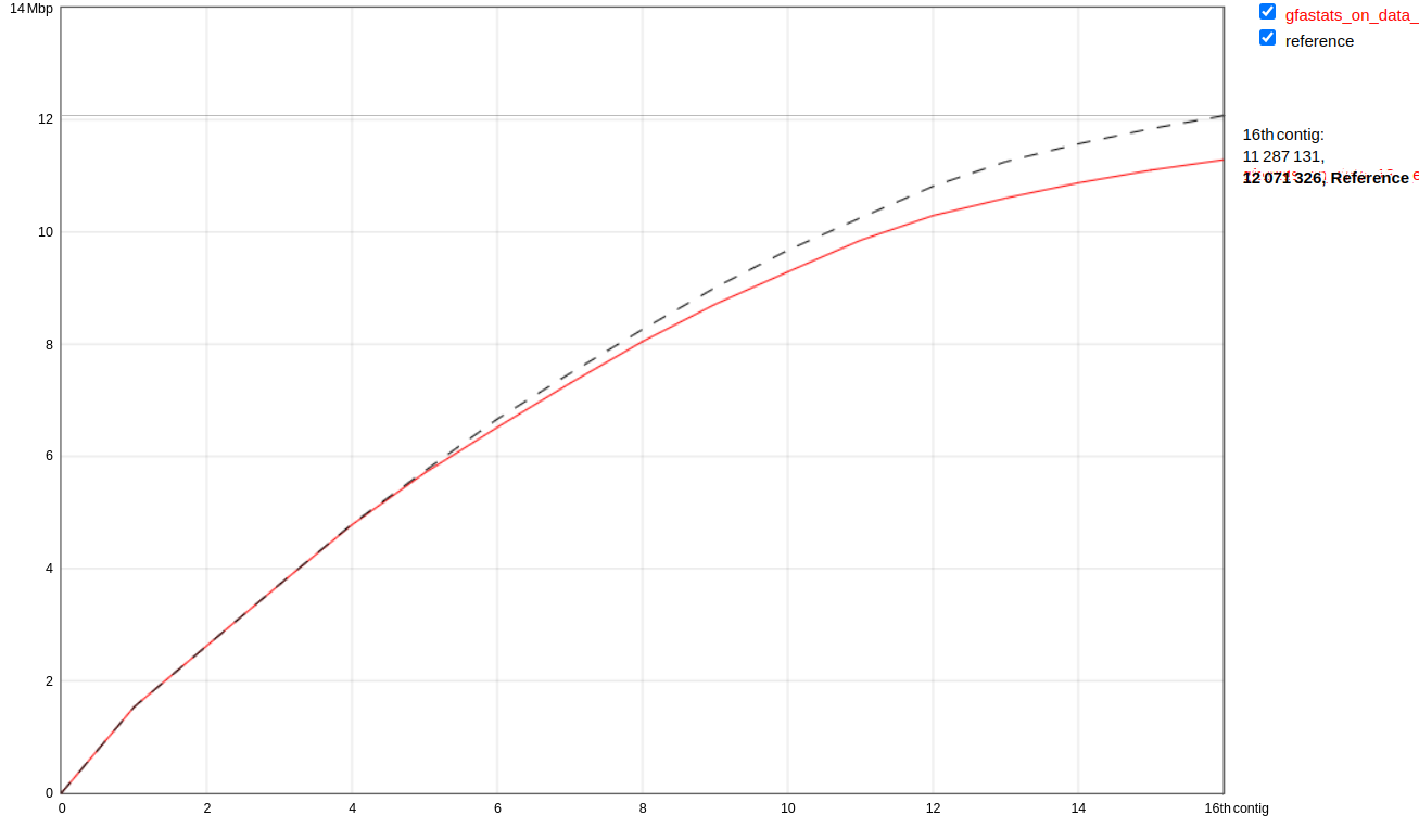
Figure 8: Cumulative continuity plot comparing assembly generated here (red line) with existing yeast reference (black dotted line). Our assembly is slightly smaller (11,304,507 bp versus 12,071,326. Our assembly is lacking the mitochondrial genome (~86 kb) because the initial data does not include mitochondrial reads. This is partially responsible for this discrepancy.
With respect to the total sequence length, we can conclude that the size of our genome assembly is very similar to the reference genome. It is noteworthy that the reference genome consists of 17 sequences, while our assembly includes only 16 chromosomes. This is due to the fact that the reference genome also includes the sequence of the mitochondrial DNA, which consists of 85,779 bp. (The above comparison is performed using Quast ( Galaxy version 5.2.0+galaxy1) using Primary assembly generated with scaffolding workflow (WF8) and yeast reference.)
Figure 9: Comparison between contact maps generated using the final Primary assembly from this tutorial (left) and the reference genome (right).
If we compare the contact map of our assembled genome with the reference assembly (Fig. above), we can see that the two are indistinguishable, suggesting that we have generated a chromosome level genome assembly.
You've Finished the Tutorial
Please also consider filling out the Feedback Form as well!
Key points
The VGP pipeline allows to generate error-free, near gapless reference-quality genome assemblies
The assembly can be divided in four main stages: genome profile analysis, HiFi long read phased assembly with hifiasm, Bionano hybrid scaffolding and Hi-C hybrid scaffolding
Frequently Asked Questions
Have questions about this tutorial? Have a look at the available FAQ pages and support channels
Simão, F. A., R. M. Waterhouse, P. Ioannidis, E. V. Kriventseva, and E. M. Zdobnov, 2015 BUSCO: assessing genome assembly and annotation completeness with single-copy orthologs. Bioinformatics 31: 3210–3212. 10.1093/bioinformatics/btv351
Ondov, B. D., T. J. Treangen, P. Melsted, A. B. Mallonee, N. H. Bergman et al., 2016 Mash: fast genome and metagenome distance estimation using MinHash. Genome biology 17: 132. 10.1186/s13059-016-0997-x
Ranallo-Benavidez, T. R., K. S. Jaron, and M. C. Schatz, 2020 GenomeScope 2.0 and Smudgeplot for reference-free profiling of polyploid genomes. Nature Communications 11: 10.1038/s41467-020-14998-3
Rhie, A., B. P. Walenz, S. Koren, and A. M. Phillippy, 2020 Merqury: reference-free quality, completeness, and phasing assessment for genome assemblies. Genome Biology 21: 10.1186/s13059-020-02134-9
Glossary
G10K
Genome 10K
GWS
Galaxy Workflow System
Hi-C
all-versus-all chromatin conformation capture
HiFi
high fidelity reads
QV
assembly consensus quality
VGP
Vertebrate Genome Project
alternate assembly
alternate loci not represented in the primary assembly
collection
Galaxy's way to represent multiple datasets as a single interface entity
collections
Galaxy's way to represent multiple datasets as a single interface entity
contigs
contiguous sequences in an assembly
primary assembly
homozygous regions of the genome plus one set of alleles for the heterozygous loci
scaffold
one or more contigs joined by gap sequence
scaffolds
one or more contigs joined by gap sequence
unitig
A uniquely assembleable subset of overlapping fragments. A unitig is an assembly of fragments for which there are no competing internal overlaps. A unitig is either a correctly assembled portion of a contig or a collapsed assembly of several high-fidelity copies of a repeat.
Feedback
Did you use this material as an instructor? Feel free to give us feedback on how it went.
Did you use this material as a learner or student? Click the form below to leave feedback.
Hiltemann, Saskia, Rasche, Helena et al., 2023 Galaxy Training: A Powerful Framework for Teaching! PLOS Computational Biology 10.1371/journal.pcbi.1010752
Batut et al., 2018 Community-Driven Data Analysis Training for Biology Cell Systems 10.1016/j.cels.2018.05.012
@misc{assembly-vgp_workflow_training,
author = "Delphine Lariviere and Alex Ostrovsky and Cristóbal Gallardo and Brandon Pickett and Linelle Abueg and Anton Nekrutenko",
	title = "Using the VGP workflows to assemble a vertebrate genome with HiFi and Hi-C data (Galaxy Training Materials)",
	year = "",
	month = "",
	day = "",
	url = "\url{https://training.galaxyproject.org/training-material/topics/assembly/tutorials/vgp_workflow_training/tutorial.html}",
	note = "[Online; accessed TODAY]"
}
@article{Hiltemann_2023,
	doi = {10.1371/journal.pcbi.1010752},
	url = {https://doi.org/10.1371%2Fjournal.pcbi.1010752},
	year = 2023,
	month = {jan},
	publisher = {Public Library of Science ({PLoS})},
	volume = {19},
	number = {1},
	pages = {e1010752},
	author = {Saskia Hiltemann and Helena Rasche and Simon Gladman and Hans-Rudolf Hotz and Delphine Larivi{\`{e}}re and Daniel Blankenberg and Pratik D. Jagtap and Thomas Wollmann and Anthony Bretaudeau and Nadia Gou{\'{e}} and Timothy J. Griffin and Coline Royaux and Yvan Le Bras and Subina Mehta and Anna Syme and Frederik Coppens and Bert Droesbeke and Nicola Soranzo and Wendi Bacon and Fotis Psomopoulos and Crist{\'{o}}bal Gallardo-Alba and John Davis and Melanie Christine Föll and Matthias Fahrner and Maria A. Doyle and Beatriz Serrano-Solano and Anne Claire Fouilloux and Peter van Heusden and Wolfgang Maier and Dave Clements and Florian Heyl and Björn Grüning and B{\'{e}}r{\'{e}}nice Batut and},
	editor = {Francis Ouellette},
	title = {Galaxy Training: A powerful framework for teaching!},
	journal = {PLoS Comput Biol}
}
Congratulations on successfully completing this tutorial!
You can use Ephemeris's shed-tools install command to install the tools used in this tutorial.
5 stars:
Liked: "Large, raw data HiFi and Hi-C can be analyzed using a stage-by-stage workflow leading to biologically meaningful data in less time.
Disliked: The addition of a brief explanation on how to launch the workflow link
June 2025
4 stars:
Liked: The workflows that are in galaxy already
Disliked: The version of the workflow is different for the assembly workflow. When you download the workflow it does not have the busco options.
January 2025
4 stars:
Liked: I liked that it was very much step by step. And the images were helpful to understand what was ment by the description.
Disliked: The workflows are not informative to understanding how they are constructed. For example, I received errors that the incorrect input data was used, but his occurred on the second Meryl job. I was not sure if this was my error or an output error of the output from the first job. Additionally, I felt like my data and histories were all over the place and I had no idea how to remove datasets from builds or move data around, then data became hidden and deleted data still existed. It would be nice to learn to navigate reorganizing histories.
August 2024
5 stars:
Liked: Very helpful to do the long pipeline with the Yeast then the short pipeline with your own data.
Disliked: In figure 7, you refer to Chub mackerel (Scomber japonicus), but then in the next sentence talk about zebra finch.
Questions:


:
Warning: Danger: Make sure you choose corect format!


Open image in new tab
 Open image in new tab
Open image in new tab
 Open image in new tab