Tuberculosis (TB) is an infectious disease caused by the bacterium Mycobacterium tuberculosis. According to the WHO, in 2018 there were 10.0 million new cases of TB worldwide and 1.4 million deaths due to the disease, making TB the world’s most deadly infectious disease. The publication of the genome of M. tuberculosis H37Rv in 1998 gave researchers a powerful new tool for understanding this pathogen. This genome has been revised since then, with the latest version being available
as RefSeq entry NC_000962.3. The genome comprises a single circular chromosome of some 4.4 megabases. The H37Rv strain that the genome was sequenced from is a long-preserved laboratory strain, originally isolated from a patient in 1905 and named as H37Rv in 1935. It is notably different in some genomic regions from some modern clinical strains but remains the standard reference sequence for M. tuberculosis (Mtb). In a larger context, M. tuberculosis is a prominent member of the Mycobacterium Tuberculosis Complex (MTBC).
This group of related species comprises the 10lineages of human-infecting M. tuberculosis as well as predominantly animal-infecting species such as M. bovis and M. pinnipedii. Two other close relatives of Mtb, M. leprae and M. lepromatosis circulate between humans, causing the disease leprosy. Finally, amongst the Mycobacteria there are several other species that live in the environment and can cause human disease. These are the Nontuberculous Mycobacteria.
Variation in the genome of M. tuberculosis (Mtb) is associated with changes in phenotype, for example, drug resistance and virulence. It is also useful for outbreak investigation as the single nucleotide polymorphisms (SNPs) in a sample can be used to build a phylogeny.
This tutorial will focus on identifying genomic variation in Mtb and using that to explore drug resistance and other aspects of the bacteria.
Get your data
The data for today is a sample of M. tuberculosiscollected from a southern African patient. In addition to the bacterial sequence sample, we will work with a Genbank format version of the genome of the inferred most recent common ancestor of the M. tuberculosis complex which is combined with the annotation of the H37Rv reference sequence. This ancestral genome only differs from the H37Rv version 3 genome (NC_000962.3) by the insertion of SNPs to try and model the ancestor of all lineages of Mtb.
Hands On: Get the data
Import the following files from Zenodo or from the shared data library
Click galaxy-uploadUpload at the top of the activity panel
Select galaxy-wf-editPaste/Fetch Data
Paste the link(s) into the text field
Press Start
Close the window
As an alternative to uploading the data from a URL or your computer, the files may also have been made available from a shared data library:
Go into Libraries (left panel)
Navigate to the correct folder as indicated by your instructor.
On most Galaxies tutorial data will be provided in a folder named GTN - Material –> Topic Name -> Tutorial Name.
Select the desired files
Click on Add to Historygalaxy-dropdown near the top and select as Datasets from the dropdown menu
In the pop-up window, choose
“Select history”: the history you want to import the data to (or create a new one)
Click on Import
Create a paired collection named Paired Reads containing the 004-2_1.fastq.gz and 004-2_2.fastq.gz datasets.
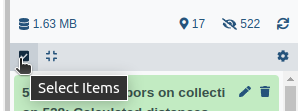
Click on galaxy-selectorSelect Items at the top of the history panel
Check all the datasets in your history you would like to include
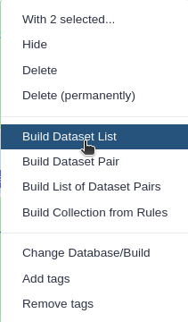
Click n of N selected and choose Advanced Build List
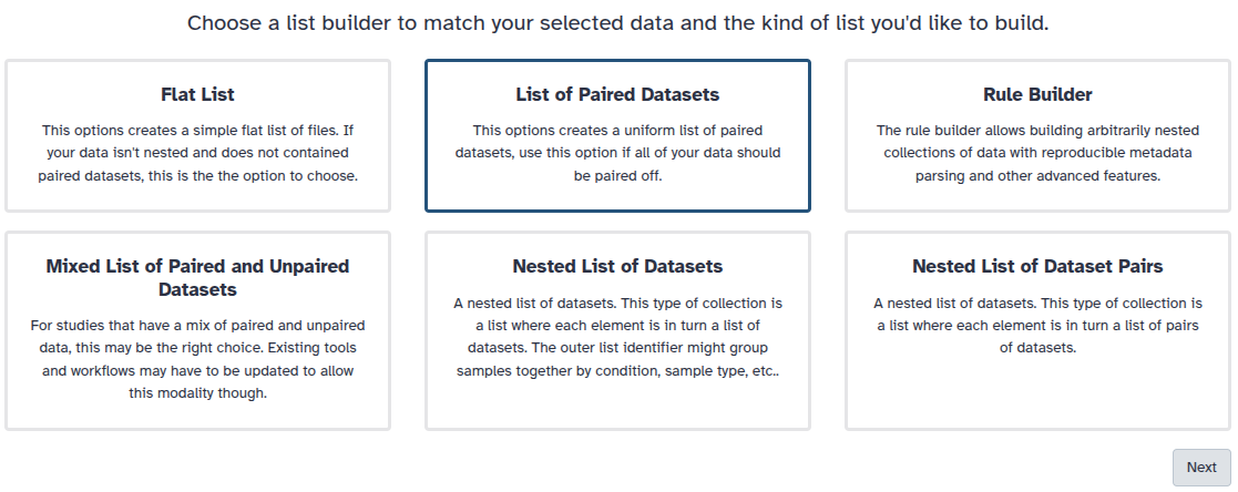
You are in the collection building wizard. Choose List of Paired Datasets and click ‘Next’ button at the right bottom corner.
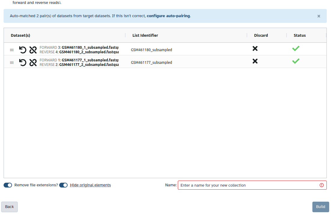
Check and configure auto-pairing. Commonly matepairs have suffix _1 and _2 or _R1 and _R2. Click on ‘Next’ at the bottom.
Edit the List Identifier as required.
Enter a name for your collection
Click Build to build your collection
Click on the checkmark icon at the top of your history again
Quality control
This step serves the purpose of identifying possible issues with the raw
sequenced reads input data before embarking on any “real” analysis steps.
Some of the typical problems with NGS data can be mitigated by preprocessing
affected sequencing reads before trying to map them to the reference genome.
Detecting some other, more severe problems early on may at least save you a lot
of time spent on analyzing low-quality data that is not worth the effort.
Here, we will perform a standard quality check on our input data and only point
out a few interesting aspects of that data. For a more thorough explanation
of NGS data quality control, you may want to have a look at the dedicated
tutorial on “Quality control”.
Hands On: Quality control of the input datasets
Run Flatten collection with the following parameters:
“Input collection”: Paired Reads
Rename the flatten collection: Flat Collection
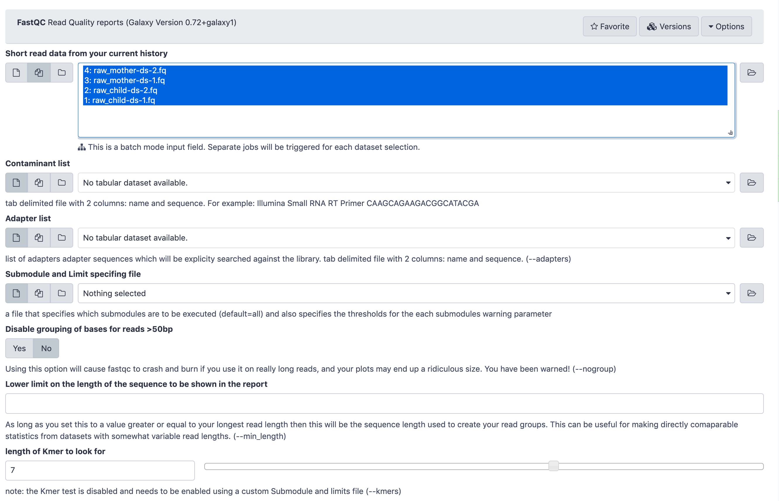
Run FastQC ( Galaxy version 0.74+galaxy1) with the following parameters:
param-collection“Raw read data from your current history”: Flat Collection (Flattened paired end read dataset collection)
The FastQCtool input form looks like this. You only need to pay attention to the top part
where Raw read data from your current history is selected. Leave all the other parameters at their default
values and click Execute.
When you start this job, four new datasets (one with the calculated raw
data, another one with an html report of the findings for each input
dataset) will get added to your history.
While one could examine the quality control report for each set of reads (forward and reverse) independently it can be quite useful to inspect them side by side using the MultiQC tool.
Hands On: Combining QC results
Use MultiQC ( Galaxy version 1.27+galaxy4) to aggregate the raw FastQC data of all input datasets into one report
In “Results”
“Which tool was used generate logs?”: FastQC
In “FastQC output”
“Type of FastQC output?”: Raw data
param-collection“FastQC output”: RawData collection output of FastQCtool
Using the galaxy-eye button, inspect the Webpage output produced by the tool
Question
Based on the report, do you think preprocessing of the reads
(trimming and/or filtering) will be necessary before mapping?
What is the average GC content of the data (known as GC%) in the 004-2_1 dataset?
Sequence quality is quite good overall. If anything you might
consider trimming the 3’ ends of reads (base qualities decline
slightly towards the 3’ ends) or to filter out the small fraction
of reads with a mean base quality < 5.
We will run fastptool on the
fastq datasets in the next step
The GC% is 66%, which is close to the 65.6% that one expects from a M. tuberculosis sample.
Examining the GC% is a quick way to check that the sample you have sequenced contains reads
from the organism that you expect.
As these reads look like they need a bit of trimming, we can turn to the fastp tool to clean up our data.
Hands On: Quality trimming
Use fastp ( Galaxy version 1.0.1+galaxy3) to clean up the reads and remove the poor quality sections.
“Single-end or paired-end reads?”: Paired Collection
“Select paired collection(s) “: Paired Reads
Inspect the output produced by fastp
Question
Was there a difference in file size of the reads before and after trimming? Is the difference the same between both sets of reads?
After processing by fastp the output files are about 80 MB smaller than the inputs. The change in size is similar for both files.
The next section, on looking for contamination in our data using Kraken2, takes a long time to run and can be skipped and perhaps
run later if you prefer.
Hands-on: Choose Your Own Tutorial
This is a 'Choose Your Own Tutorial' (CYOT) section (also known as 'Choose Your Own Analysis' (CYOA)), where you can select between multiple paths. Click one of the buttons below to select how you want to follow the tutorial
Look for contamination with Kraken2
We should also look for contamination in our reads. Sometimes, other sources of DNA accidentally or inadvertently get mixed in with our sample. Any reads from non-sample sources will confound our SNP analysis. Kraken2 is an effective way of looking at which species is represented in our reads so we can easily spot possible contamination of our sample. Unfortunately, the tool uses a lot of RAM (typically 50GB when used with the Standard database), so you might want to skip this step if your environment doesn’t have enough computing nodes able to process such jobs. For an example of a probably-contaminated sample that does not use Kraken2 as part of its analysis, see the optional section on analysing SRR12416842 at the end of this tutorial.
Hands On: Run Kraken2
Execute Kraken2 ( Galaxy version 2.17.1+galaxy0) with the following parameters
“Single or paired reads”: Paired
“Collection of paired reads”: fastp on X: Paired-end output
“Print scientific names instead of just taxids”: Yes
“Enable quick operation”: Yes
“Print a report with aggregrate counts/clade to file”: Yes
“Select a Kraken2 database”: Standard
Inspect the report produced by Kraken
Question
Was there any significant contamination of the sample?
Over 85% of the reads here have been positively identified as Mycobacterium (the precise % will differ depending on which version of the Kraken database you are using). The others found were bacteria from the same kingdom. There were no contaminating human or viral sequences detected.
Find variants with Snippy
We will now run the Snippy tool on our reads, comparing them to the reference.
Snippy is a tool for rapid bacterial SNP calling and core genome alignments. Snippy finds SNPs between a haploid reference genome and your NGS sequence reads. It will find both substitutions (SNPs) and insertions/deletions (indels).
If we give Snippy an annotated reference in Genbank format, it will run a tool called SnpEff which will figure out the effect of any changes on the genes and other features. If we just give Snippy the reference sequence alone without the annotations, it will not run SnpEff.
We have an annotated reference built from the inferred M. tuberculosisancestral reference genome and the
gene annotation from the H37Rv strain so will use it in this case.
Hands On: Run Snippy
Snippy ( Galaxy version 4.6.0+galaxy0) with the following parameters
“Will you select a reference genome from your history or use a built-in index?”: Use a genome from history and build index
“Use the following dataset as the reference sequence”: Mycobacterium_tuberculosis_ancestral_reference.gbk
“Input type”: Paired end reads in a collection
“Select a paired collection”: fastp on X: Paired-end output
Under “Advanced parameters”
“Minimum proportion for variant evidence”: 0.1 (This is so we can see possible rare variants in our sample)
Under “Output selection” select the following:
“The final annotated variants in VCF format”
“A simple tab-separated summary of all the variants”
“The alignments in BAM format”
Deselect any others.
Inspect the Snippy VCF output
Question
What type of variant is the first one in the list?
What was the effect of this variant on the coding region it was found in?
How many variants were found?
Substitution of a C to a T. This variant is supported by 197 reads.
According to SnpEff, it’s a Synonymous change in Rv0002.
1098 variants are found. To count variants, look at how many non-comment lines are in the snippy VCF output or how many lines (excluding the header) there are in the VCF file. This is quite typical for M. tuberculosis.
RECAP: So far we have taken our sample reads, cleaned them up a bit, checked for taxonomic assocation, compared the reads with our reference sequence and then called variants (SNPs and indels) between our sample and the reference genome. We have tried to mitigate a few errors along the way:
Sequencing errors: these were addressed by the quality trimming step
Sample contamination: we used Kraken2 to assess the extent of this problem in our sample
Appropriate choice of a reference genome: we used a genome that is inferred to be ancestral to all M. tuberculosis for our analysis and the diversity within Mtb is limited enough for us to rely on a single reference genome for the entire species.
Quality filtering in the mapping and variant calling stage: Internally snippy uses tools like bwa-mem and freebayes that judge the quality of their predictions. snippy then uses this information to perform some filtering on variant calling predictions.
Further variant filtering and drug resistance profiling
We still cannot entirely trust the proposed variants. In particular, there are regions of the M. tuberculosis genome that are difficult to effectively map reads to. These include the PE/PPE/PGRS genes, which are highly repetitive, and the IS (insertion sequence sites). Secondly, when an insertion or deletion (indel) occurs in our sample relative to the reference it can cause apparent, but false, single nucleotide variants to appear near the indel. Finally, where few reads map to a region of the reference genome, either because of a sequence deletion or because of a high GC content in the genomic region, we cannot be confident about the quality of variant calling in the region. The TB Variant Filter can help filter out variants based on a variety of criteria, including those listed above.
Hands On: Run TB Variant Filter
TB Variant Filter ( Galaxy version 0.4.0+galaxy0) with the following parameters
“VCF file to be filter”: snippy on collection XX snps vcf file
“Filters to apply”: Select Filter variants by region and Filter sites by read alignment depth.
Open the new VCF file.
Question
How many of the original variants have now been filtered out?
131 (The difference in the number of lines between the snippy vcf file and the filtered vcf file.)
TB Variant Filter tries to provide reasonable defaults for filtering
variants predicted in the M. tuberculosis
genome, using multiple different strategies.
Firstly, certain regions of the Mtb genome
contain repetitive sequences, e.g. from
the PE/PPE gene family. Historically all of the genomic regions corresponding to
those genes were filtered out but
the new default draws on work from
Maximillian Marin and others. This
list of “refined low confidence” (RLC)
regions is the current region filter in
TB Variant Filter for reads over 100 bp.
If you are using shorter reads (e.g. from Illumina iSeq) the “Refined Low Confidence and Low Mappability” region list should be used instead.
For more on how these regions were calculated read the paper or preprint.
In addition to region filters, filters for variant type, allele frequency, coverage depth and distance from indels are provided.
Older variant callers struggled to accurately
call insertions and deletions (indels) but more recent tools (e.g. GATK v4 and the variant caller used in Snippy, Freebayes) no longer have this weakness. One remaining reason to filter SNVs/SNPs near indels is that they might have a different
evolutionary history to “free standing” SNVs/SNPs, so the “close to indel filter” is still available in TB Variant Filter in case such SNPs/SNVs should be filtered out.
Now that we have a collection of high-quality variants we can search them against variants known to be associated with drug resistance. The TB Profiler tool does this using a database of variants curated by Dr Jody Phelan at the London School of Hygiene and Tropical Medicine. It can do its own mapping and variant calling but also accepts mapped reads in BAM format as input. It does its own variant calling and filtering.
Finally, TB Variant Report uses the COMBAT-TB eXplorerdatabase of M. tuberculosis genome annotation to annotate variants in Mtb. It also takes the output of TB Profiler and produces a neat report that is easy to browse and search.
Hands On: Run TB Profiler and TB Variant Report
TB-Profiler profile ( Galaxy version 6.6.4+galaxy0) with the following parameters
“Input File Type”: BAM
“Bam”: snippy on collection XX mapped reads (bam)
TB Profiler produces 3 output files, it’s own VCF file, a report about the sample including it’s likely lineages and any AMR found. There is also a .json formatted results file.
When snippy is run with Genbank format input it prepends GENE_ to gene names in the VCF annotation. This causes a problem for TB Variant report, so we need to edit the output with sed.
Text transformation with sed ( Galaxy version 9.5+galaxy2) with the following parameters:
“File to process”: TB Variant Filter on data XX
“SED Program”: s/GENE_//g
TB Variant Report ( Galaxy version 1.0.1+galaxy0) with the following parameters
“Input SnpEff annotated M.tuberculosis VCF(s)”: Text transformation on data XX
“TBProfiler Drug Resistance Report (Optional)”: TB-Profiler Profile on data XX: Results.json
Open the drug resistance and variant report html files.
Question
What was the final lineage of the sample we tested?
Were there any drug resistances found?
4 with sublineage 4.4.1.1.1.
Yes, resistance to isoniazid, rifampicin, ethambutol, pyrazinamide and streptomycin as well as to the flouroquinolines (amikacin, capreomycin and kanamycin) is predicted from mutations in the katG, rpoB, embB, pncA, rpsL and rrs (ribosomal RNA) genes respectively.
At this point we have a drug resistance report from TB Profiler, aligned reads from snippy and variants both in VCF format
and in the easier-to-read format produced by TB Variant report. Often this is enough information on a sample, and we might end
our analysis here, especially if we are processing many samples together, as is described towards the end of this tutorial.
We will, however, spend some time examining this data in more detail in the next section.
View Snippy output in JBrowse
We could go through all of the variants in the VCF files and read them out of a text table, but this is onerous and doesn’t really give the context of the changes very well. It would be much nicer to have a visualisation of the SNPs and the other relevant data. A genome viewer, such as JBrowse, can be used within Galaxy to display the M. tuberculosis genome and the data from our analysis.
Hands On: Run JBrowse
Use seqret ( Galaxy version 5.0.0) to convert the Genbank format reference (Mycobacterium_tuberculosis_ancestral_reference.gbk) to FASTA format. Use the following parameters:
JBrowse ( Galaxy version 1.16.11+galaxy1) with the following parameters
“Reference genome to display”: Use a genome from history
“Select the reference genome”: seqret output from the previous step
This sequence will be the reference against which annotations are displayed
“Genetic Code”: 11: The Bacterial, Archaeal and Plant Plastid Code
“JBrowse-in-Galaxy Action”: New JBrowse Instance
“Track Group”
We will now set up three different tracks - these are datasets displayed underneath the reference sequence (which is displayed as nucleotides in FASTA format). We will choose to display the sequence reads (the .bam file), the variants found by snippy (the .gff file) and the annotated reference genome (the wildtype.gff)
Track 1 - sequence reads: Click on Insert Track Group and fill it with
“Track Category” to sequence reads
Click on Insert Annotation Track and fill it with
“Track Type” to BAM Pileups
“BAM Track Data” to snippy on collection XX mapped reads (bam)
“Autogenerate SNP Track” to No
“Track Visibility” to On for new users
Track 2 - variants: Click on Insert Track Group and fill it with
“Track Category” to variants
Click on Insert Annotation Track and fill it with
“Track Type” to VCF SNPs
“SNP Track Data” to TB Variant Filter on data XX
“Track Visibility” to On for new users
Track 3 - annotated reference: Click on Insert Track Group and fill it with
“Track Category” to annotated reference
Click on Insert Annotation Track and fill it with
“Track Type” to GFF/GFF3/BED Features
“GFF/GFF3/BED Track Data” to Mycobacterium_tuberculosis_h37rv.ASM19595v2.45.chromosome.Chromosome.gff3
“JBrowse Track Type [Advanced]” to Canvas Features
Click on “JBrowse Styling Options [Advanced]”
“JBrowse style.label” to product
“JBrowse style.description” to product
“Track Visibility” to On for new users
A new dataset will be created in your history, containing the JBrowse interactive visualisation. We will now view its contents and play with it by clicking the galaxy-eye (eye) icon of the JBrowse on data XX and data XX - Complete dataset. The JBrowse window will appear in the centre Galaxy panel.
You can now click on the names of the tracks to add them in, try the vcf file and gff file. You can see where the variants are located and which genes they are in. If you click on the BAM file you can zoom right in to see the read alignments for each variant if you wish.
Question: Using JBrowse to examine a known variant
Paste Chromosome:761009..761310 into the JBrowse location bar and click Go. Ensure that the BAM and VCF tracks are set to visible. What is the meaning of the red column that shows up in the middle of the display of reads (the BAM track)?
What change happened at position 761155 in the genome, according to the read and variant data displayed?
How did this change impact the rpoB gene, the gene that is found on the forward strand overlapping this position?
The red column is a variant that is present in almost all of the reads aligning to the genome at position 761155.
Examining the VCF track the variant is shown as a mutation from C to T.
The “frame” of the codons in this gene can be determined by navigating to where the rpoB gene, the second horizontal bar in the annotation track, starts (position 759807). This gene is in frame 0 on the forward strand, the top frame in the display. Navigating back to position 761155, the amino acid encoded in the reference genome is S, that is serine. The mutation from a C to a T changes the codon at this position to L, leucine, and is associated with resistance to the drug rifampicin.
While the rifampicin resistance mutation being examined here is already reported by TB-Profiler, JBrowse allows us to examine the evidence underlying this mutation in more detail.
An alternative to running JBrowse within Galaxy is to install IGV and use Galaxy’s built-in support for visualising BAM files with IGV.
You can send data from your Galaxy history to IGV for viewing as follows:
In recent versions of IGV, you will have to enable the port:
In IGV, go to View > Preferences > Advanced
Check the box Enable Port
In Galaxy, expand the dataset you would like to view in IGV
Make sure you have set a reference genome/database correctly (dbkey) (instructions)
Under display in IGV, click on local
This requires more setup for the user, for example loading the FASTA file of the genome into IGV and downloading any annotation GFF3 files you want to use with IGV. On the other hand, running IGV locally is often faster than using JBrowse in Galaxy.
Different samples, different stories (optional)
In Zenodo we have included sample 18-1 from the same study (aka. ERR1750907). This is also a southern African
M. tuberculosis sample, but in some ways quite different from the sample we have analysed in the tutorial thus
far.
Examine the sequence quality with FastQC ( Galaxy version 0.74+galaxy1).
Examine the sample composition with Kraken2 ( Galaxy version 2.17.1+galaxy0).
Question
What problems were discovered with sequence quality?
What did the Kraken2 report show? How does this impact your assessment of variants discovered from this sample?
The quality of the sequence drops sharply towards the end of the sequences. Even more concerning, the sequence content changes across the length of the sample, which is not what we would expect at all. Finally, the sample seems to contain sequencing adapters, an artefact of the sequencing process that should be trimmed out before any sequence analysis.
Less than 60% of the sequence reads are associated with the genus Mycobacterium. Perhaps the quality problems in the sequence reads contribute to this poor classification? They certainly will make variant calling less reliable. You might get too many (false positive) or too few (false negative) variants reported compared to what is actually present in the sample.
As you can see, the quality of sequence data strongly determines how useful it is for subsequent analysis. This is why quality control is always a first step before trying to call and interpret variants. What we do with a sample like this will depend on what resources we have available. Can we discard it and use other data for our analysis? Can we re-sequence? Can we clean it up, remove the adapters (using Trimmomatic, fastp or cutadapt) and perhaps use the Kraken2 output to decide which reads to keep? These are all possible strategies and there is no one answer for which is the correct one to pursue.
The next example is SRR12416842 from an Indonesia study of multi-drug resistant (MDR) tuberculosis.
Hands On: Take a closer look at sample SRR12416842
Fetch the data from EBI European Nucleotide Archive
Perform quality trimming with fastp ( Galaxy version 1.0.1+galaxy3) and examine it’s HTML output to see quality before and after trimming.
Map the samples to the M. tuberculosis reference genome with Snippy ( Galaxy version 4.6.0+galaxy0). Make sure to select the BAM output as one of the outputs.
Question
Was the sequence quality good?
How many variants were discovered by snippy?
The fastp result shows that while there is some dropoff in sequence quality (especially towards the end of the reads from the second dataset), the sequences are of good enough quality to analyse.
snippy discovered more than 15,000 variants. This is unusual for a M. tuberculosis sample where we expect at most a few thousand variants across the length of the genome.
Run samtools stats ( Galaxy version 2.0.8) on the snippy on collection XX mapped reads (bam) file. In the output, pay attention to the sequences, reads mapped and reads unmapped results.
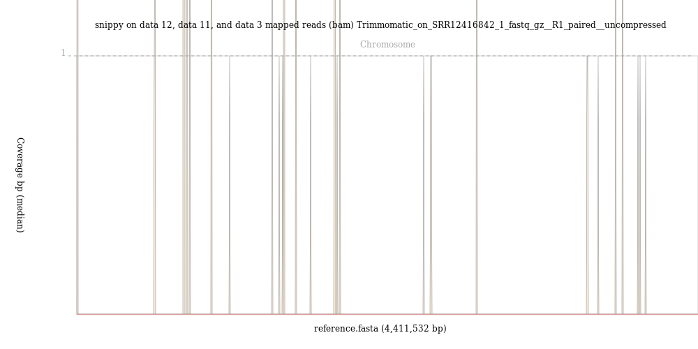
Run the BAM Coverage Plotter ( Galaxy version 20201223+galaxy0) on the mapped reads BAM file that you got from snippy using the FASTA format reference you made with seqret as the reference.
Question
What percentage of reads mapped to the reference genome?
If you could run the BAM Coverage Plotter tool, was the coverage even across the genome?
Less than 110000 out of 7297618, that is 1.5%, of the reads mapped to the reference genome.
The image from the BAM Coverage Plotter tool shows just a few vertical bars, suggestion that almost no reads mapped to the reference genome.
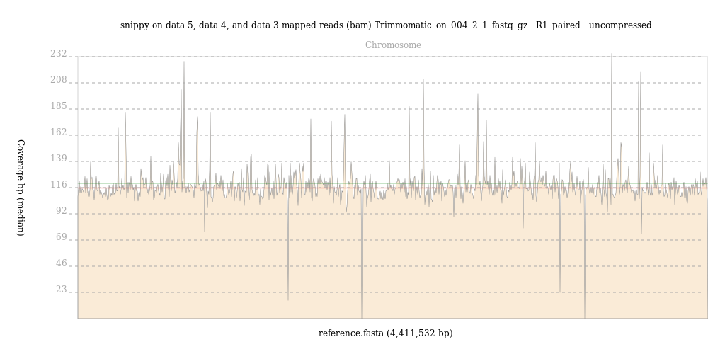
By contrast, reads from the 004-02 map evenly across the M. tuberculosis genome, with an average depth of over 100 reads, as shown in this output from BAM Coverage Plotter:
If you wish to investigate further, analyse the SRR12416842 sample with Kraken2.
There is something clearly wrong with sample SRR12416842, perhaps indicating sample contamination. This example of a sample that doesn’t map to the reference genome illustrates that even when sequence quality is good, sequence data problems can become apparent in later steps of analysis and it is important to always have a sense of what results to expect. You can develop a better sense of what quality control results to expect by first practicing techniques with known data before analysing new samples.
Processing many samples at once: Collections and Workflows (optional)
In the tutorial thus far we have focused on processing single samples, where two read datasets (forward and reverse reads) are associated with a single sample. In practice, sequence analysis typically involves analysing batches of samples and we run the same
analysis steps for each sample in the batch. Galaxy supports working with batches using collections and workflows.
If you have followed all of the steps of this tutorial, you will have two useable samples, one named 004-2 and another 018-1. Create a list of dataset pairs from these samples and call the collection samples.
Click on galaxy-selectorSelect Items at the top of the history panel
Check all the datasets in your history you would like to include
Click n of N selected and choose Advanced Build List
You are in the collection building wizard. Choose List of Paired Datasets and click ‘Next’ button at the right bottom corner.
Check and configure auto-pairing. Commonly matepairs have suffix _1 and _2 or _R1 and _R2. Click on ‘Next’ at the bottom.
Edit the List Identifier as required.
Enter a name for your collection
Click Build to build your collection
Click on the checkmark icon at the top of your history again
The workflow that we are going to use is published on WorkflowHub.eu and you can run it directly on Galaxy servers using the link below:
Hands On: Importing and Launching a WorkflowHub.eu Workflow
Click on galaxy-workflows-activityWorkflows in the Galaxy activity bar (on the left side of the screen, or in the top menu bar of older Galaxy instances). You will see a list of all your workflows
Click on galaxy-uploadImport at the top-right of the screen
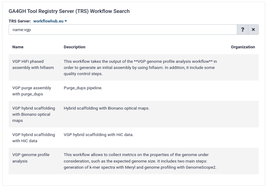
On the new page, select the GA4GH servers tab, and configure the GA4GH Tool Registry Server (TRS) Workflow Search interface as follows:
“TRS Server”: workflowhub.eu
“search query”: name:"TB Variant Analysis v1.0"
Expand the correct workflow by clicking on it
Select the version you would like to galaxy-upload import
The workflow will be imported to your list of workflows. Note that it will also carry a little blue-white shield icon next to its name, which indicates that this is an original workflow version imported from a TRS server. If you ever modify the workflow with Galaxy’s workflow editor, it will lose this indicator.
Below is a short video showing the entire uncomplicated procedure:
Video: Importing via search from WorkflowHub
If the text above doesn’t show a text to run or if you are not on one of the public “usegalaxy.*” servers that integrate with WorkflowHub.eu:
Copy the URL of this link (e.g. via right click) or save it to your computer and
Import the workflow into Galaxy
Click the run icon (it is a small white right-pointing triangle on a blue background)
Click on galaxy-workflows-activityWorkflows in the Galaxy activity bar (on the left side of the screen, or in the top menu bar of older Galaxy instances). You will see a list of all your workflows
Click on galaxy-uploadImport at the top-right of the screen
Provide your workflow
Option 1: Paste the URL of the workflow into the box labelled “Archived Workflow URL”
Option 2: Upload the workflow file in the box labelled “Archived Workflow File”
Click the Import workflow button
Below is a short video demonstrating how to import a workflow from GitHub using this procedure:
Video: Importing a workflow from URL
Hands On: Analysing samples with the TB Variant Reporting workflow
Run the TB Variant Analysis workflowworkflow using the following parameters
param-collectionReads the samples collection of your input reads
param-fileReference Genome the Mycobacterium_tuberculosis_ancestral_reference.gbk reference genome
Click the Run Workflow button at the top-right of the screen
The workflow will produce a series of collections, with the most important outputs being tagged with dataset tags.
The MultiQC report tagged qc_report contains information on fastp read trimming and BamQC mapping statistics.
The filtered VCF is transformed with sed and tagged as annotated_vcf
The TB-Profiler drug resistance report is tagged with drug_resistance_report
The TB VCF Report outputs are tagged with variant_report
For each sample a consensus genome is created by inserting the single nucleotide variants into the reference genome. This is tagged as consensus_genome and is intended for use in building a phylogenetic tree.
The Kraken2 report (to check for contamination) is tagged with kraken_report
The workflow also produces a Workflow Invocation Report that summarises the outputs of the workflow. This can be found on the Workflow Invocation menu which is either in the User menu or on the History menu depending on which version of Galaxy you are using.
Conclusion
Thank you for coming to the end of this tutorial. After completing this tutorial you might want to follow some of the other tutorials in the Galaxy Training Network on analysing M. tuberculosis data. Just search for tuberculosis in the search bar. Enjoy the rest of your day!
You've Finished the Tutorial
Please also consider filling out the Feedback Form as well!
Key points
variants in M. tuberculosis sequencing data can be discovered using common microbial bioinformatics tools
it is not enough to just call variants, variant calling involves multiple quality control steps
the choice of reference genome and some quality control procedures are species-specific, and require knowledge of the organism in question
batches of samples can be processed using Galaxy dataset collections and workflows
Frequently Asked Questions
Have questions about this tutorial? Have a look at the available FAQ pages and support channels
Further information, including links to documentation and original publications, regarding the tools, analysis techniques and the interpretation of results described in this tutorial can be found here.
Feedback
Did you use this material as an instructor? Feel free to give us feedback on how it went.
Did you use this material as a learner or student? Click the form below to leave feedback.
Hiltemann, Saskia, Rasche, Helena et al., 2023 Galaxy Training: A Powerful Framework for Teaching! PLOS Computational Biology 10.1371/journal.pcbi.1010752
Batut et al., 2018 Community-Driven Data Analysis Training for Biology Cell Systems 10.1016/j.cels.2018.05.012
@misc{variant-analysis-tb-variant-analysis,
author = "Peter van Heusden and Simon Gladman and Thoba Lose",
	title = "M. tuberculosis Variant Analysis (Galaxy Training Materials)",
	year = "",
	month = "",
	day = "",
	url = "\url{https://training.galaxyproject.org/training-material/topics/variant-analysis/tutorials/tb-variant-analysis/tutorial.html}",
	note = "[Online; accessed TODAY]"
}
@article{Hiltemann_2023,
	doi = {10.1371/journal.pcbi.1010752},
	url = {https://doi.org/10.1371%2Fjournal.pcbi.1010752},
	year = 2023,
	month = {jan},
	publisher = {Public Library of Science ({PLoS})},
	volume = {19},
	number = {1},
	pages = {e1010752},
	author = {Saskia Hiltemann and Helena Rasche and Simon Gladman and Hans-Rudolf Hotz and Delphine Larivi{\`{e}}re and Daniel Blankenberg and Pratik D. Jagtap and Thomas Wollmann and Anthony Bretaudeau and Nadia Gou{\'{e}} and Timothy J. Griffin and Coline Royaux and Yvan Le Bras and Subina Mehta and Anna Syme and Frederik Coppens and Bert Droesbeke and Nicola Soranzo and Wendi Bacon and Fotis Psomopoulos and Crist{\'{o}}bal Gallardo-Alba and John Davis and Melanie Christine Föll and Matthias Fahrner and Maria A. Doyle and Beatriz Serrano-Solano and Anne Claire Fouilloux and Peter van Heusden and Wolfgang Maier and Dave Clements and Florian Heyl and Björn Grüning and B{\'{e}}r{\'{e}}nice Batut and},
	editor = {Francis Ouellette},
	title = {Galaxy Training: A powerful framework for teaching!},
	journal = {PLoS Comput Biol}
}
Funding
These individuals or organisations provided funding support for the development of this resource
4 stars:
Liked: Find variants with Snippy and filtering, plotting drug resistance
Disliked: Further details in the practical examples
5 stars:
Liked: The TB variant analysis workflow
Disliked: I would like to persuade my Director about the protection of institutional data on Galaxy. How is raw data protected on the server, and for how long? When data is deleted in the user space, is this deletion permanent? Who else has the right to view the data and delete it permanently, apart from the user, if the platform is saturated? Thank you
June 2025
5 stars:
Liked: The workflow that was imported is mindblowing! It's literally an end-to-end analysis of Mtb isolates.
5 stars:
Liked: I liked the simple instructions that were not too descriptive and screen shots of how the tools and how entries would/should appear
Disliked: The part on JBrowse seemed a bit complicated for the hands-on tutorial. This needs more clarification.
5 stars:
Disliked: I found the tutorial too long to complete at once, maybe it could be diveded into two.
4 stars:
Liked: i like the fact that the whole process was easy to follow and the interpretations came in handy
July 2024
3 stars:
Liked: I was able to challenge myself, and had a background knowledge of how to determine SNPs and drug resistance patterns
Disliked: Some of the version IDs don't tally with the version provided for the tutorial
June 2024
5 stars:
Liked: The sequential flow of the work makes it easier to understand downstream analysis using Galaxy. I practiced this tutorial three times, and I have conceptualized the key aspect of mapping and variant calling for Mtb NGS analysis.
Disliked: How to translate this knowledge and skills in analyzing NGS raw data for Enteric pathogens and other microorganisms. Please, for comparative data analysis, you can add one ESKAPE pathogen for this studies
4 stars:
Liked: The step-by-step analysis of the genome. Very interesting information and easy to follow steps. I like Galaxy. The course was well organized and really made easy for people like me who is a wet lab scientist who is not familiar with the dry lab analysis and computer systems.
Disliked: I think next time, the time should be extended to allow the participants to complete all the tutorials before moving to the next session. The reason I am saying this is because from my own personal experience, it is difficult to pay attention in the next session when your mind is still stuck in the previous tutorial that was left incomplete. other that, the course was well organized and really made easy for people like me who is a wet lab scientist.
5 stars:
Liked: Gene viewing, Find variants with Snippy
Disliked: probably direct the us the new users to run tool after commanding
5 stars:
Liked: The hints section since the galaxy platform is new to me. I am used to coding and using the linux platform. But this was refreshing to use
Disliked: An example comparing single-end and paired-end data results would be interesting
5 stars:
Liked: Stepwise presentation of information made it easy to follow the tutorial
Disliked: Please, the training has been more productive. You can include information on genotyping Mycobacterium ulceran to give a clear-cut genomic differences between Mtb
5 stars:
Liked: Presentation skills, audibility of the instructor
4 stars:
Liked: step by step guide
Disliked: I did not get the same JBrowse so I tried to do it again. I still got the "minimal" instead of the "complete" even after following the step by step procedure.
October 2023
4 stars:
Liked: Very clear and well explain tutorial
Disliked: Maybe I would suggest to put some figures to easy find some commands on galaxy
May 2023
5 stars:
Liked: Have a great Job. I am doing my Research on MTB of Bioinformatics Analysis. It was really Helpful.
Disliked: sorry to say, but one of my suggestion is on next time need Hands on Session Tutorial vedio.
January 2023
5 stars:
Liked: The extra examples (2 NGS datasets) at the end of the tutorial are very useful, it gives me a better idea on how to troubleshoot and identify the problem, when encountering a bad NGS data
Disliked: Perhaps it will be helpful to include more explanation of the results for the different tools after each steps (e.g. a hyperlink to the bioinformatics tool's user manual for more result explanation)
July 2022
4 stars:
Liked: The clear instructions on how to use the tools
Disliked: allowing learners to supply the solution and evaluating the answers
March 2022
5 stars:
Liked: Tutorials easy to follow
Disliked: This is great model of learning
4 stars:
Liked: I like that even though we do not have to type in commands, we still have steps to follow. I have made errors but still were able to use tools to rectify. One can play around till the correct output!
Disliked: Specification of version to use as we ended up getting different answers due to using default version
Questions: