Because this tutorial consists of many steps, we have made two versions of it, one long and one short.
This is the shortened version. Instead of running each tool individually, we will employ
workflows to run groups of analysis steps (e.g. data cleaning) at once. If you would like
more in-depth discussion of each step, please see the longer version of tutorial
You can also switch between the long and short version at the start of any section.
Your results may be slightly different from the ones presented in this tutorial due to differing versions of tools, reference data, external databases, or because of stochastic processes in the algorithms.
Obtaining and preparing data
In this tutorial we use 16S rRNA data, but similar pipelines can be used for WGS data.
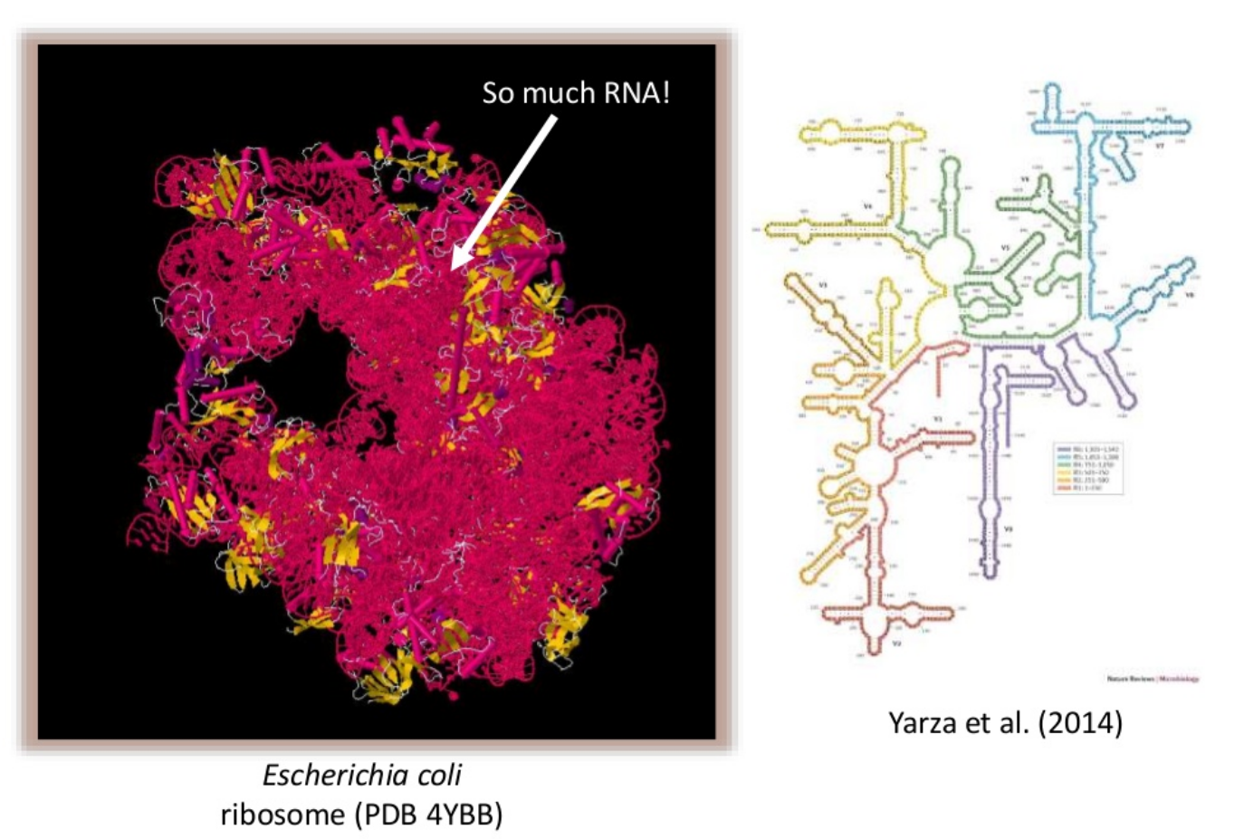
Comment: Background: The 16S ribosomal RNA gene
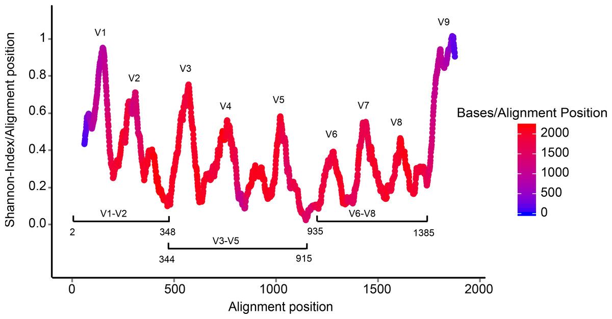
The 16S rRNA gene has several properties that make it ideally suited for our purposes
Present in all prokaryotes
Highly conserved + highly variable regions
Huge reference databases
The highly conserved regions make it easy to target the gene across different organisms,
while the highly variable regions allow us to distinguish between different species.
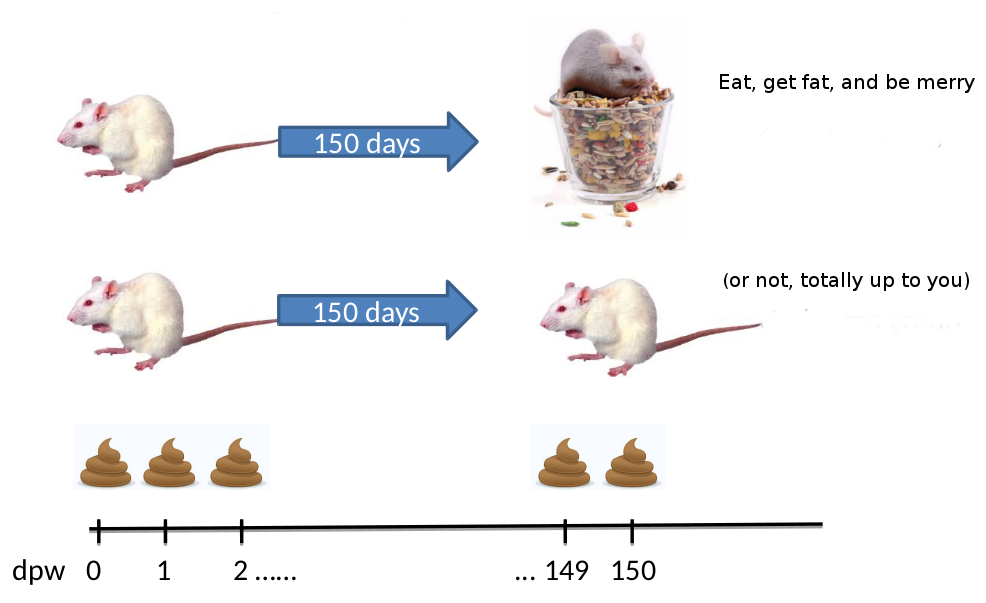
“The Schloss lab is interested in understanding the effect of normal variation in the gut microbiome on host health. To that end,
we collected fresh feces from mice on a daily basis for 365 days post weaning. During the first 150 days post weaning (dpw),
nothing was done to our mice except allow them to eat, get fat, and be merry. We were curious whether the rapid change in
weight observed during the first 10 dpw affected the stability microbiome compared to the microbiome observed between days
140 and 150.”
To speed up analysis for this tutorial, we will use only a subset of this data. We will look at a single mouse at 20 different
time points (10 early, 10 late). In order to assess the error rate of the analysis pipeline and experimental setup, the Schloss lab
additionally sequenced a mock community with a known composition (genomic DNA from 21 bacterial strains). The sequences used
for this mock sample are contained in the file HMP_MOCK.v35.fasta
Comment: Dataset naming scheme
For this tutorial, you are given 20 pairs of files. For example, the following pair of files: F3D0_R1.fastq F3D0_R2.fastq
The first part of the file name indicates the sample; F3D0 here signifies that this sample was obtained from Female 3 on Day 0.
The _R1 and _R2 are used to indicate the forward and reverse reads respectively.
Importing the data into Galaxy
Now that we know what our input data is, let’s get it into our Galaxy history:
All data required for this tutorial has been made available from Zenodo
Hands On: Obtaining our data
Make sure you have an empty analysis history. Give it a name.
To create a new history simply click the new-history icon at the top of the history panel:
Import Sample Data.
Import the sample FASTQ files to your history, either from a shared data library (if available), or from Zenodo
using the URLs listed in the box below (click param-repeat to expand):
Now that’s a lot of files to manage. Luckily Galaxy can make life a bit easier by allowing us to create
dataset collections. This enables us to easily run tools on multiple datasets at once.
Since we have paired-end data, each sample consist of two separate fastq files, one containing the
forward reads, and one containing the reverse reads. We can recognize the pairing from the file names,
which will differ only by _R1 or _R2 in the filename. We can tell Galaxy about this paired naming
convention, so that our tools will know which files belong together. We do this by building a List of Dataset Pairs
Hands On: Organizing our data into a paired collection
Create a paired collection named Mouse samples,
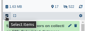
Click on galaxy-selectorSelect Items at the top of the history panel
Check all the datasets in your history you would like to include
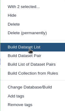
Click n of N selected and choose Advanced Build List
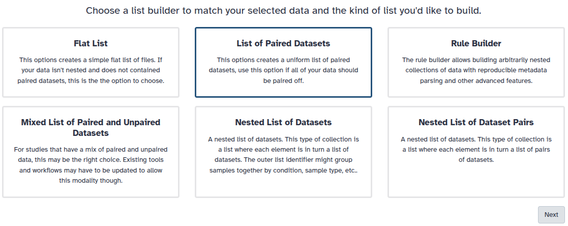
You are in the collection building wizard. Choose List of Paired Datasets and click ‘Next’ button at the right bottom corner.
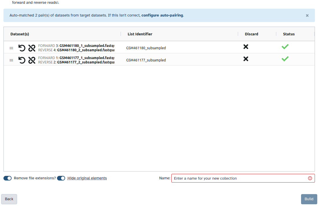
Check and configure auto-pairing. Commonly matepairs have suffix _1 and _2 or _R1 and _R2. Click on ‘Next’ at the bottom.
Edit the List Identifier as required.
Enter a name for your collection
Click Build to build your collection
Click on the checkmark icon at the top of your history again
Comment
Make sure that param-checkRemove file extensions is checked
Check that the pairs are named F3D0-F3D9, F3D141-F3D150 and Mock.
Note: The names should not have the .fastq extension
If needed, the names can be edited manually by clicking on them
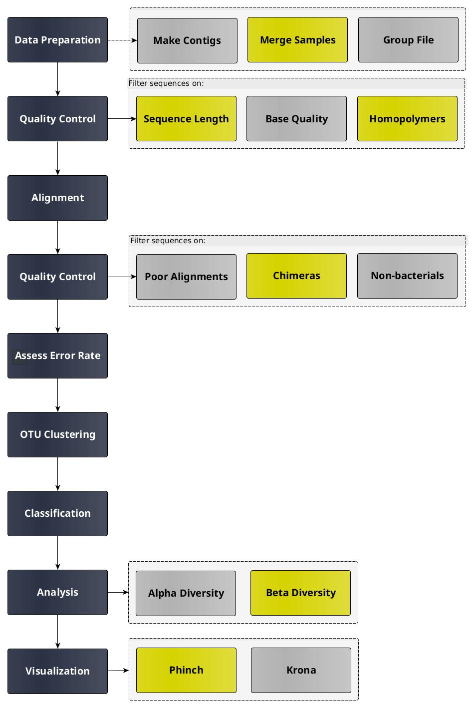
Before starting any analysis, it is always a good idea to assess the quality of your input data and improve it
where possible by trimming and filtering reads. The mothur toolsuite contains several tools to assist with this task.
We will begin by merging our reads into contigs, followed by filtering and trimming of reads based on quality score
and several other metrics.
Create contigs from paired-end reads
In this experiment, paired-end sequencing of the ~253 bp V4 region of the 16S rRNA gene was performed.
The sequencing was done from either end of each fragment. Because the reads are about 250 bp in length, this results in a
significant overlap between the forward and reverse reads in each pair. We will combine these pairs of reads into contigs.
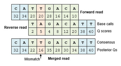
The Make.contigs tool creates the contigs, and uses the paired collection as input. Make.contigs
will look at each pair, take the reverse complement reverse read, and then determine the overlap between the
two sequences. Where an overlapping base call differs between the two reads, the quality score is used to determine
the consensus base call. A new quality score is derived by combining the two original quality scores in both of
the reads for all the overlapping positions.
Hands On: Combine forward and reverse reads into contigs
Make.contigs ( Galaxy version 1.39.5.1) with the following parameters
param-select“Way to provide files”: Multiple pairs - Combo mode
param-collection“Fastq pairs”: the collection you just created
Leave all other parameters to the default settings
This step combined the forward and reverse reads for each sample, and also combined
the resulting contigs from all samples into a single file. So we have gone from a paired
collection of 20x2 FASTQ files, to a single FASTA file. In order to retain information about
which reads originated from which samples, the tool also output a group file. View that
file now, it should look something like this:
Here the first column contains the read name, and the second column contains the sample name.
Data Cleaning
Next, we want to improve the quality of our data. To this end we will run a workflow that performs the following steps:
Filter by length
We know that the V4 region of the 16S gene is around 250 bp long. Anything significantly longer
was likely a poorly assembled contig. We will remove any contigs longer than 275 base pairs using the Screen.seqstool tool.
Remove low quality contigs
We will also remove any contigs containing too many ambiguous base calls. This is also done in the Screen.seqstool tool.
Deduplicate sequences
Since we are sequencing many of the same organisms, there will likely be many identical contigs. To speed up downstream analysis we will determine the set of unique contigs using Unique.seqstool.
Counting sequences
Finally we count how often each of the unique sequences occurs in the given samples. These counts are stored in the count_table.
Click on galaxy-workflows-activityWorkflows in the Galaxy activity bar (on the left side of the screen, or in the top menu bar of older Galaxy instances). You will see a list of all your workflows
Click on galaxy-uploadImport at the top-right of the screen
Paste the following URL into the box labelled “Archived Workflow URL”: https://training.galaxyproject.org/training-material/topics/microbiome/tutorials/mothur-miseq-sop-short/workflows/workflow1_quality_control.ga
Click the Import workflow button
Below is a short video demonstrating how to import a workflow from GitHub using this procedure:
Video: Importing a workflow from URL
Run Workflow 1: Quality Controlworkflow using the following parameters:
“Send results to a new history”: No
param-file“1: Contigs”: the trim.contigs.fasta output from Make.contigstool
param-file“2: Groups”: the group file from Make.contigstool
param-text“3: max seq len”: Set a maximum sequence length of 275
Click on Workflows on the Activity Bar on the left.
At the top of the resulting page you will have the option to switch between the My workflows, Workflows shared with me and Public workflows tabs.
Select the tab you want to see all workflows in that category
Search for your desired workflow.
Click on the workflow name: a pop-up window opens with a preview of the workflow.
To run it directly: click Run (top-right).
Recommended: click Import (left of Run) to make your own local copy under Workflows / My Workflows.
Question
How many sequences were removed in the screening step?
How many unique sequences are there in our cleaned dataset?
The screening removed 23,488 sequences.
This can be determined by looking at the number of lines in bad.accnos output of Screen.seqstool
or by comparing the total number of sequences before and after this screening step in the output of Summary.seqstool
There are 16,426 unique sequences.
This can be determined by expanding one of the outputs of Unique.seqstool and looking at the number of lines in the file.
Have a look at the count_table output from the Count.seqstool, it summarizes the number of times each unique sequence was observed across each of the samples. It will look something like this:
The first column contains the read names of the representative sequences, and the subsequent columns contain
the number of duplicates of this sequence observed in each sample.
Comment: Representative sequences vs Total sequences
From now on, we will only work with the set of unique sequences, but it’s important to remember that these represent a larger
number of total sequences, which we keep track of in the count table.
In the following we will use the unique sequences together with the count table as input to tools instead of the complete set of sequences. If this is done for the Summary.seqstool tool it will
report both the number of unique representative sequences as well as the total sequences they represent.
We are now ready to align our sequences to the reference alignment. This is an important
step to improve the clustering of your OTUs Schloss 2012.
In mothur this is done by determining for each unique sequence the entry of the reference database that
has the most k-mers in common (i.e. the most substring of fixed length k). For the reference sequence
with the most common k-mers and the unique sequence a standard global sequence alignment is computed
(using the Needleman-Wunsch algorithm).
Hands On: Align sequences
Align.seqs ( Galaxy version 1.39.5.0) with the following parameters
param-file“fasta”: the fasta output from Unique.seqstool
param-file“reference”: silva.v4.fasta reference file from your history
Question
Have a look at the alignment output, what do you see?
At first glance, it might look like there is not much information there. We see our read names, but only period . characters below it.
This is because the V4 region is located further down our reference database and nothing aligns to the start of it. If you scroll to right you will start seeing some more informative bits:
.....T-------AC---GG-AG-GAT------------
Here we start seeing how our sequences align to the reference database.
There are different alignment characters in this output:
.: terminal gap character (before the first or after the last base in our query sequence)
-: gap character within the query sequence
We will cut out only the V4 region in a later step (Filter.seqstool)
Summary.seqs ( Galaxy version 1.39.5.0) with the following parameters:
param-file“fasta”: the align output from Align.seqstool
param-file“count”: count_table output from Count.seqstool
The Start and End columns tell us that the majority of reads aligned between positions 1968 and 11550,
which is what we expect to find given the reference file we used. However, some reads align to very different positions,
which could indicate insertions or deletions at the terminal ends of the alignments or other complicating factors.
Also notice the Polymer column in the output table. This indicates the average homopolymer length. Since we know that
our reference database does not contain any homopolymer stretches longer than 8 reads, any reads containing such
long stretches are likely the result of PCR errors and we would be wise to remove them.
Next we will clean our data further by removing poorly aligned sequences and any sequences with long
homopolymer stretches.
More Data Cleaning
To ensure that all our reads overlap our region of interest, we will:
Remove any reads not overlapping the region V4 region using Screen.seqstool.
Remove any overhang on either end of the V4 region to ensure our sequences overlap only the V4 region, using Filter.seqstool.
Clean our alignment file by removing any columns that have a gap character (-, or . for terminal gaps) at that position in every sequence (also using Filter.seqstool).
Remove redundancy in the aligned sequences that might have been introduced by filtering columns by running Unique.seqs once more.
Group near-identical sequences together with Pre.clustertool. Sequences that only differ by one or two bases at this point are likely to represent sequencing errors rather than true biological variation, so we will cluster such sequences together.
Remove Sequencing artefacts known as chimeras (discussed in next section) from the counts file using Chimera.vsearch and from the fasta file with remove.seqs.
Chimera Removal
During PCR amplification, it is possible that two unrelated templates are combined to form a sort of hybrid sequence,
also called a chimera. Needless to say, we do not want such sequencing artefacts confounding our results. We’ll do
this chimera removal using the VSEARCH algorithm Rognes et al. 2016 that is called within mothur, using the
Chimera.vsearchtool tool.
Click on galaxy-workflows-activityWorkflows in the Galaxy activity bar (on the left side of the screen, or in the top menu bar of older Galaxy instances). You will see a list of all your workflows
Click on galaxy-uploadImport at the top-right of the screen
Paste the following URL into the box labelled “Archived Workflow URL”: https://training.galaxyproject.org/training-material/topics/microbiome/tutorials/mothur-miseq-sop-short/workflows/workflow2_data_cleaning.ga
Click the Import workflow button
Below is a short video demonstrating how to import a workflow from GitHub using this procedure:
Video: Importing a workflow from URL
Run Workflow 2: Data Cleaning and Chimera Removalworkflow using the following parameters:
“Send results to a new history”: No
param-file“1: Aligned Sequences”: the align output from Align.seqstool
param-file“2: Count Table”: the count table from Count.seqstool
Click on Workflows on the Activity Bar on the left.
At the top of the resulting page you will have the option to switch between the My workflows, Workflows shared with me and Public workflows tabs.
Select the tab you want to see all workflows in that category
Search for your desired workflow.
Click on the workflow name: a pop-up window opens with a preview of the workflow.
To run it directly: click Run (top-right).
Recommended: click Import (left of Run) to make your own local copy under Workflows / My Workflows.
Question
How many chimeric sequences were detected?
How many sequences remain after these cleaning steps?
There were 3,467 representative sequences flagged as chimeric. These represent a total of 10,827 total sequences
This can be determined by looking at the number of sequences in the vsearch.accnos file (3,467). To determine how many total sequences these represent, compare the Summary.seqs log output files before and after the chimera filtering step (128,872-118,045=10,827).
There are 2,264 remaining sequences after filtering, clustering of highly similar sequences, and chimera removal.
This can be determined by looking at the number of sequences in the fasta output of Remove.seqstool
Have a look at the FASTA output from Pre.cluster, it should looks something like this:
We see that these are our contigs, but with extra alignment information. The filtering steps have removed any positions which had a gap symbol in all reads of the dataset.
Now that we have thoroughly cleaned our data, we are finally ready to assign a taxonomy to our sequences.
We will do this using a Bayesian classifier (via the Classify.seqstool tool) and a mothur-formatted training
set provided by the Schloss lab based on the RDP (Ribosomal Database Project, Cole et al. 2013) reference taxonomy.
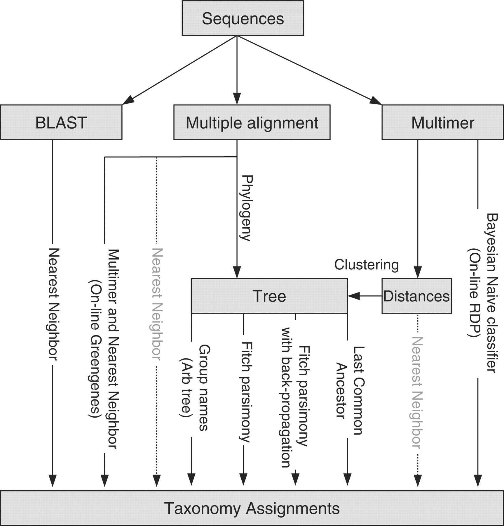
Comment: Background: Taxonomic assignment
In this tutorial we will use the RDP classifier and reference taxonomy for classification, but there are several different taxonomic
assignment algorithms and reference databases available for this purpose.
An overview of different methods is given by Liu et al. 2008 and shown below:
The choice of taxonomic classifier and reference taxonomy can impact downstream results. The figure from Liu et al. 2008
given below shows the taxonomic composition determined when using different classifiers and reference taxonomies, for different primer sets (16S regions).
Figure: Compositions at the phylum level for each of the three datasets: (a) Guerrero Negro mat, (b) Human gut and (c) Mouse gut, using a range of different methods (separate subpanels within each group). The x-axis of each graph shows region sequenced. The y-axis shows abundance as a fraction of the total number of sequences in the community. The legend shows colors for phyla (consistent across graphs).
Which reference taxonomy is best for your experiments depends on a number of factors such as the type of sample and variable region sequenced.
Another discussion about how these different databases compare was described by Balvočiūtė and Huson 2017.
Removal of non-bacterial sequences
Despite all we have done to improve data quality, there may still be more to do:
there may be 18S rRNA gene fragments or 16S rRNA from Archaea, chloroplasts, and mitochondria
that have survived all the cleaning steps up to this point. We are generally not interested in these sequences
and want to remove them from our dataset.
Hands On: Taxonomic Classification and removal of non-bacterial sequences
Click on galaxy-workflows-activityWorkflows in the Galaxy activity bar (on the left side of the screen, or in the top menu bar of older Galaxy instances). You will see a list of all your workflows
Click on galaxy-uploadImport at the top-right of the screen
Paste the following URL into the box labelled “Archived Workflow URL”: https://training.galaxyproject.org/training-material/topics/microbiome/tutorials/mothur-miseq-sop-short/workflows/workflow3_classification.ga
Click the Import workflow button
Below is a short video demonstrating how to import a workflow from GitHub using this procedure:
Video: Importing a workflow from URL
Run Workflow 3: Classificationworkflow using the following parameters:
“Send results to a new history”: No
param-file“1: Cleaned sequences”: the fasta output from Remove.seqs (i.e. pick.fasta) tool
param-file“2: Count Table”: the count table from Remove.seqs (i.e. pick.count) tool
param-file“3: Training set Taxonomy”: trainset9_032012.pds.tax file you imported from Zenodo
param-file“4: Training set FASTA”: trainset9_032012.pds.fasta file from Zenodo
Click on Workflows on the Activity Bar on the left.
At the top of the resulting page you will have the option to switch between the My workflows, Workflows shared with me and Public workflows tabs.
Select the tab you want to see all workflows in that category
Search for your desired workflow.
Click on the workflow name: a pop-up window opens with a preview of the workflow.
To run it directly: click Run (top-right).
Recommended: click Import (left of Run) to make your own local copy under Workflows / My Workflows.
Question
How many non-bacterial sequences were removed? Determine both the number of representative sequences and total sequences removed.
There were 20 representative sequences removed, representing 162 total sequences.
This can be determined by looking at the summary.seqs log outputs before the Remove.lineage step (after chimera removal), and after.
The data is now as clean as we can get it. In the next section we will use the Mock sample to assess how accurate
our sequencing and bioinformatics pipeline is.
Optional: Calculate error rates based on our mock community
The mock community analysis is optional. If you are low on time or want to skip ahead, you can jump straight to the next section
where we will cluster our sequences into OTUs, classify them and perform some visualisations.
If you wish to skip the mock community analysis, you can go directly to the next section and continue with the analysis.
The following step is only possible if you have co-sequenced a mock community with your samples. A mock community is a sample
of which you know the exact composition and is something we recommend to do, because it will give you an idea of how
accurate your sequencing and analysis protocol is.
Comment: Background: Mock communities
What is a mock community?
A mock community is an artificially constructed sample; a defined mixture of microbial cells and/or
viruses or nucleic acid molecules created in vitro to simulate the composition of a microbiome
sample or the nucleic acid isolated therefrom.
Why sequence a mock community?
In a mock community, we know exactly which sequences/organisms we expect to find, and at which proportions.
Therefore, we can use such an artificial sample to assess the error rates of our sequencing and
analysis pipeline.
Did we miss any of the sequences we know to be present in the sample (false negatives)?
Do we find any sequences that were not present in the sample (false positives)?
Were we able to accurately detect their relative abundances?
If our workflow performed well on the mock sample, we have more confidence in the accuracy of the
results on the rest of our samples.
Example
As an example, consider the following image from Fouhy et al Fouhy et al. 2016.
A mock community sample was sequenced for different combinations of sequencer and primer sets (V-regions).
Since we know the expected outcome, we can assess the accuracy of each pipeline. A similar approach can be used to
assess different parameter settings of the in-silico analysis pipeline.
Figure 1: Example of usage of a mock community to assess accuracy. On the left is the expected result given that we know the exact composition of the mock sample. This was then used to assess the accuracy of different combinations of sequencing platform and primer set (choice of V-region)
Further reading
Next generation sequencing data of a defined microbial mock community Singer et al. 2016
16S rRNA gene sequencing of mock microbial populations- impact of DNA extraction method, primer choice and sequencing platform Fouhy et al. 2016
The mock community in this experiment was composed of genomic DNA from 21 bacterial strains. So in a perfect world, this is
exactly what we would expect the analysis to produce as a result.
First, let’s extract the sequences belonging to our mock samples from our data:
Hands On: extract mock sample from our dataset
Get.groups ( Galaxy version 1.39.5.0) with the following parameters
param-file“group file or count table”: the count table from Remove.lineagetool
param-select“groups”: Mock
param-file“fasta”: fasta output from Remove.lineagetool
param-check“output logfile?”: yes
In the log file we see the following:
Selected 58 sequences from your fasta file.
Selected 4046 sequences from your count file
The Mock sample has 58 unique sequences, representing a total of 4,046 total sequences.
The Seq.error tool measures the error rates using our mock reference. Here we align
the reads from our mock sample back to their known sequences, to see how many fail to match.
Hands On: Assess error rates based on a mock community
Seq.error ( Galaxy version 1.39.5.0) with the following parameters
param-file“fasta”: the fasta output from Get.groupstool
param-file“reference”: HMP_MOCK.v35.fasta file from your history
param-file“count”: the count table from Get.groupstool
That is pretty good! The error rate is only 0.0065%! This gives us confidence that the rest of the samples
are also of high quality, and we can continue with our analysis.
Cluster mock sequences into OTUs
We will now estimate the accuracy of our sequencing and analysis pipeline by clustering the Mock sequences into OTUs,
and comparing the results with the expected outcome.
For this a distance matrix is calculated (i.e. the distances between all pairs of sequences). From this distance matrix
a clustering is derived using the OptiClust algorithm:
OptiClust starts with a random OTU clustering
Then iteratively sequences are moved to all other OTUs or new clusters and the option is chosen that improved the mathews correlation coefficient (MCC)
Step 2 is repeated until the MCC converges
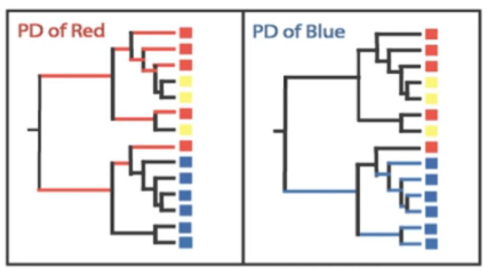
Comment: Background: What are Operational Taxonomic Units (OTUs)?
In 16S metagenomics approaches, OTUs are clusters of similar sequence variants of the 16S rDNA marker gene
sequence. Each of these clusters is intended to represent a taxonomic unit of a bacteria species or genus
depending on the sequence similarity threshold. Typically, OTU cluster are defined by a 97% identity
threshold of the 16S gene sequence variants at species level. 98% or 99% identity is suggested for strain
separation.
(Image credit: Danzeisen et al. 2013, 10.7717/peerj.237)
Click on galaxy-workflows-activityWorkflows in the Galaxy activity bar (on the left side of the screen, or in the top menu bar of older Galaxy instances). You will see a list of all your workflows
Click on galaxy-uploadImport at the top-right of the screen
Paste the following URL into the box labelled “Archived Workflow URL”: https://training.galaxyproject.org/training-material/topics/microbiome/tutorials/mothur-miseq-sop-short/workflows/workflow4_mock_otu_clustering.ga
Click the Import workflow button
Below is a short video demonstrating how to import a workflow from GitHub using this procedure:
Video: Importing a workflow from URL
Run Workflow 4: Mock OTU Clusteringworkflow using the following parameters:
“Send results to a new history”: No
param-file“1: Mock Count Table”: the count table output from Get.groupstool
param-file“2: Mock Sequences”: the fasta output from Get.groupstool
Click on Workflows on the Activity Bar on the left.
At the top of the resulting page you will have the option to switch between the My workflows, Workflows shared with me and Public workflows tabs.
Select the tab you want to see all workflows in that category
Search for your desired workflow.
Click on the workflow name: a pop-up window opens with a preview of the workflow.
To run it directly: click Run (top-right).
Recommended: click Import (left of Run) to make your own local copy under Workflows / My Workflows.
Question
How many OTUs were identified in our mock community?
Answer: 34
This can be determined by opening the shared file or OTU list and looking at the header line. You will see a column for each OTU
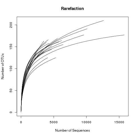
Open the rarefaction output (dataset named sobs inside the rarefaction curves output collection), it should look
something like this:
When we use the full set of 4060 sequences, we find 34 OTUs from the Mock community; and with
3000 sequences, we find about 31 OTUs. In an ideal world, we would find exactly 21 OTUs. Despite our
best efforts, some chimeras or other contaminations may have slipped through our filtering steps.
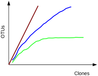
Comment: Background: Rarefaction
To estimate the fraction of species sequenced, rarefaction curves are typically used. A rarefaction curve
plots the number of species as a function of the number of individuals sampled. The curve usually begins
with a steep slope, which at some point begins to flatten as fewer species are being discovered per sample:
the gentler the slope, the less contribution of the sampling to the total number of operational taxonomic
units or OTUs.
Green, most or all species have been sampled; blue, this habitat has not been exhaustively sampled; red,
species rich habitat, only a small fraction has been sampled.
In this tutorial we will continue with an OTU-based approach, for the phylotype and phylogenic
approaches, please refer to the mothur wiki page.
Comment: Background: What are Operational Taxonomic Units (OTUs)?
In 16S metagenomics approaches, OTUs are clusters of similar sequence variants of the 16S rDNA marker gene
sequence. Each of these clusters is intended to represent a taxonomic unit of a bacteria species or genus
depending on the sequence similarity threshold. Typically, OTU cluster are defined by a 97% identity
threshold of the 16S gene sequence variants at species level. 98% or 99% identity is suggested for strain
separation.
(Image credit: Danzeisen et al. 2013, 10.7717/peerj.237)
We will now repeat the OTU clustering we performed on our mock community for our real datasets. We use a slightly different workflow because these tools are faster for larger datasets. We will also normalize our data by subsampling to the level of the sample with the lowest number of sequences in it.
Click on galaxy-workflows-activityWorkflows in the Galaxy activity bar (on the left side of the screen, or in the top menu bar of older Galaxy instances). You will see a list of all your workflows
Click on galaxy-uploadImport at the top-right of the screen
Paste the following URL into the box labelled “Archived Workflow URL”: https://training.galaxyproject.org/training-material/topics/microbiome/tutorials/mothur-miseq-sop-short/workflows/workflow5_otu_clustering.ga
Click the Import workflow button
Below is a short video demonstrating how to import a workflow from GitHub using this procedure:
Video: Importing a workflow from URL
Run Workflow 5: OTU Clusteringworkflow using the following parameters:
“Send results to a new history”: No
param-file“1: Sequences”: the fasta output from Remove.lineagetool
param-file“2: Count table”: the count table output from Remove.lineagetool
param-file“3: Taxonomy”: the taxonomy output from Remove.lineagetool
Click on Workflows on the Activity Bar on the left.
At the top of the resulting page you will have the option to switch between the My workflows, Workflows shared with me and Public workflows tabs.
Select the tab you want to see all workflows in that category
Search for your desired workflow.
Click on the workflow name: a pop-up window opens with a preview of the workflow.
To run it directly: click Run (top-right).
Recommended: click Import (left of Run) to make your own local copy under Workflows / My Workflows.
Examine galaxy-eye the taxonomy output of Classify.otutool. This is a collection, and the different levels of taxonomy are shown in the names of the collection elements. In this example we only calculated one level, 0.03. This means we used a 97% similarity threshold. This threshold is commonly used to differentiate at species level.
Opening the taxonomy output for level 0.03 (meaning 97% similarity, or species level) shows a file structured like the following:
The first line shown in the snippet above indicates that Otu008 occurred 5258 times, and that all of the
sequences (100%) were binned in the genus Alistipes.
Question
Which samples contained sequences belonging to an OTU classified as Staphylococcus?
Examine the tax.summary file output by Classify.otutool.
Samples F3D141, F3D142, F3D144, F3D145, F3D2. This answer can be found by
examining the tax.summary output and finding the columns with nonzero
values for the line of Staphylococcus
Before we continue, let’s remind ourselves what we set out to do. Our original question was about the stability of
the microbiome and whether we could observe any change in community structure between the early and late samples.
Species diversity is a valuable tool for describing the ecological complexity of a single sample (alpha diversity)
or between samples (beta diversity). However, diversity is not a physical quantity that can be measured directly,
and many different metrics have been proposed to quantify diversity by Finotello et al. 2016.
Comment: Background: Species Diversity
Species diversity consists of three components: species richness, taxonomic or phylogenetic diversity and species evenness.
Species richness = the number of different species in a community.
Species evenness = how even in numbers each species in a community is.
Phylogenetic diversity = how closely related the species in a community are.
Each of these factors play a role in diversity, but how to combine them into a single measure of diversity is nontrivial.
Many different metrics have been proposed for this, for example: shannon, chao, pd, ace, simpson, sobs, jack, npshannon,
smithwilson, heip bergerparker, boney, efron, shen, solow, bootstrap, qstat, coverage, anderberg, hamming, jclass, jest,
ochiai, canberra, thetayc, invsimpson, just to name a few ;). A comparison of several different diversity metrics is discussed in Bonilla-Rosso et al. 2012
Question
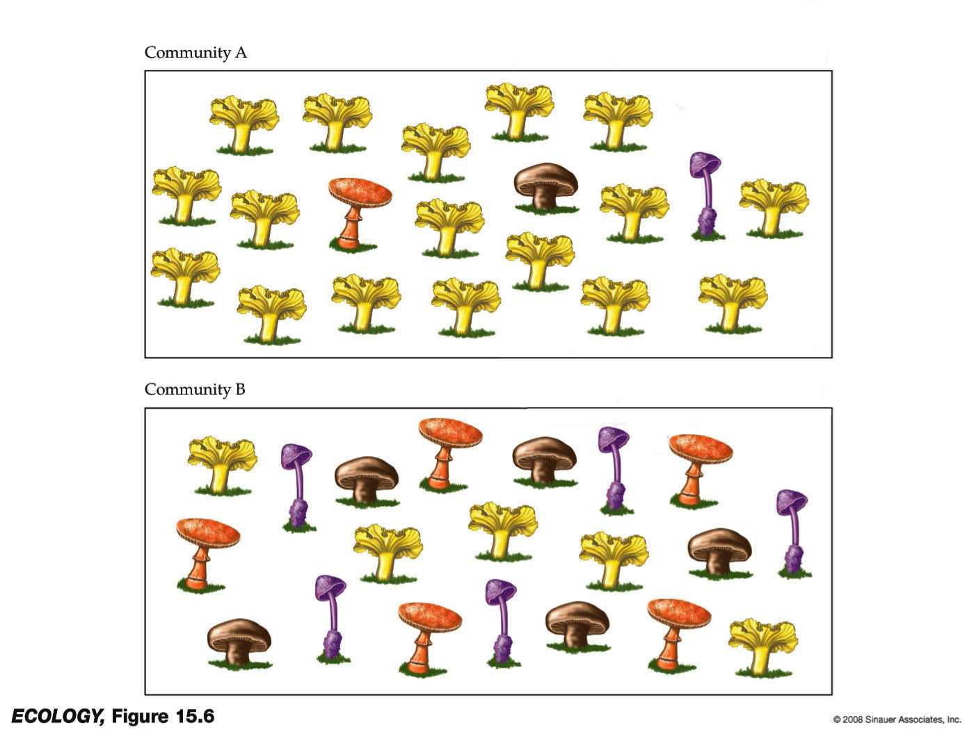
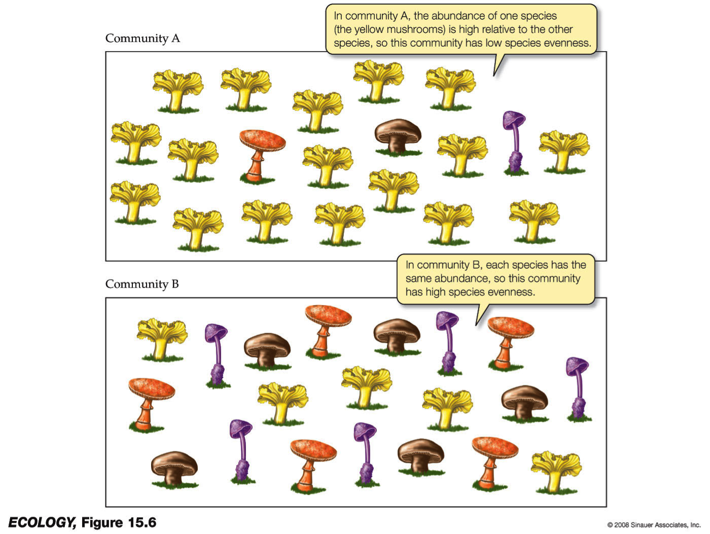
To understand the difference between richness and evenness, consider the following example:
Which of these communities has the highest richness?
Which of these communities has the highest evenness?
Both communities have 4 different species, so they have same richness.
Community B is more even, because each species has the same abundance.
Even when two samples have identical richness and evenness, we still may conclude that one is more diverse than
the other if the species are very dissimilar in one of the samples (have high phylogenetic distance), but very
closely related to each other in the second sample.
Now, you do not need to know what all these different metrics are, but just remember that there is not a single
definition of diversity and as always, the metric you choose to use may influence your results.
Alpha diversity
In order to estimate alpha diversity of the samples, we first generate the rarefaction curves. Recall that
rarefaction measures the number of observed OTUs as a function of the subsampling size.
Comment: Background: Rarefaction
To estimate the fraction of species sequenced, rarefaction curves are typically used. A rarefaction curve
plots the number of species as a function of the number of individuals sampled. The curve usually begins
with a steep slope, which at some point begins to flatten as fewer species are being discovered per sample:
the gentler the slope, the less contribution of the sampling to the total number of operational taxonomic
units or OTUs.
Green, most or all species have been sampled; blue, this habitat has not been exhaustively sampled; red,
species rich habitat, only a small fraction has been sampled.
We will use a plotting tool to visualize the rarefaction curves, and use Summary.singletool to calculate a number of different alpha diversity metrics on all our samples.
Click on galaxy-workflows-activityWorkflows in the Galaxy activity bar (on the left side of the screen, or in the top menu bar of older Galaxy instances). You will see a list of all your workflows
Click on galaxy-uploadImport at the top-right of the screen
Paste the following URL into the box labelled “Archived Workflow URL”: https://training.galaxyproject.org/training-material/topics/microbiome/tutorials/mothur-miseq-sop-short/workflows/workflow6_alpha_diversity.ga
Click the Import workflow button
Below is a short video demonstrating how to import a workflow from GitHub using this procedure:
Video: Importing a workflow from URL
Run Workflow 6: Alpha Diversityworkflow using the following parameters:
“Send results to a new history”: No
param-file“1: Shared File”: the Shared file output from Make.sharedtool
Click on Workflows on the Activity Bar on the left.
At the top of the resulting page you will have the option to switch between the My workflows, Workflows shared with me and Public workflows tabs.
Select the tab you want to see all workflows in that category
Search for your desired workflow.
Click on the workflow name: a pop-up window opens with a preview of the workflow.
To run it directly: click Run (top-right).
Recommended: click Import (left of Run) to make your own local copy under Workflows / My Workflows.
View the rarefaction plot output. From this image can see that the rarefaction curves for all samples have started to level
off so we are confident we cover a large part of our sample diversity:
View the summary output from Summary.singletool. This shows several alpha diversity metrics:
The differences in diversity and richness between early and late time points is small.
All sample coverage is above 97%.
There are many more diversity metrics, and for more information about the different calculators available in mothur, see the mothur wiki page
We could perform additional statistical tests (e.g. ANOVA) to confirm our feeling that there is no significant difference based on sex or early vs. late, but this is beyond the scope of this tutorial.
Beta diversity
Beta diversity is a measure of the similarity of the membership and structure found between different samples.
The default calculator in the following section is thetaYC, which is the Yue & Clayton theta similarity
coefficient. We will also calculate the Jaccard index (termed jclass in mothur).
In the following workflow we will:
Calculate pairwise distances between samples using the thetaYC calculator (Dist.sharedtool)
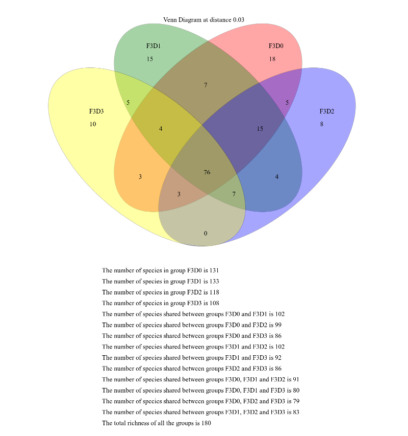
Create a Venn diagram to show the number of overlapping OTUs between 4 of our samples
Create a heatmap of the intersample similarities (Heatmap.simtool)
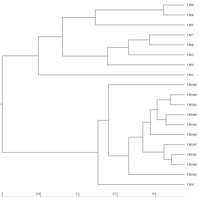
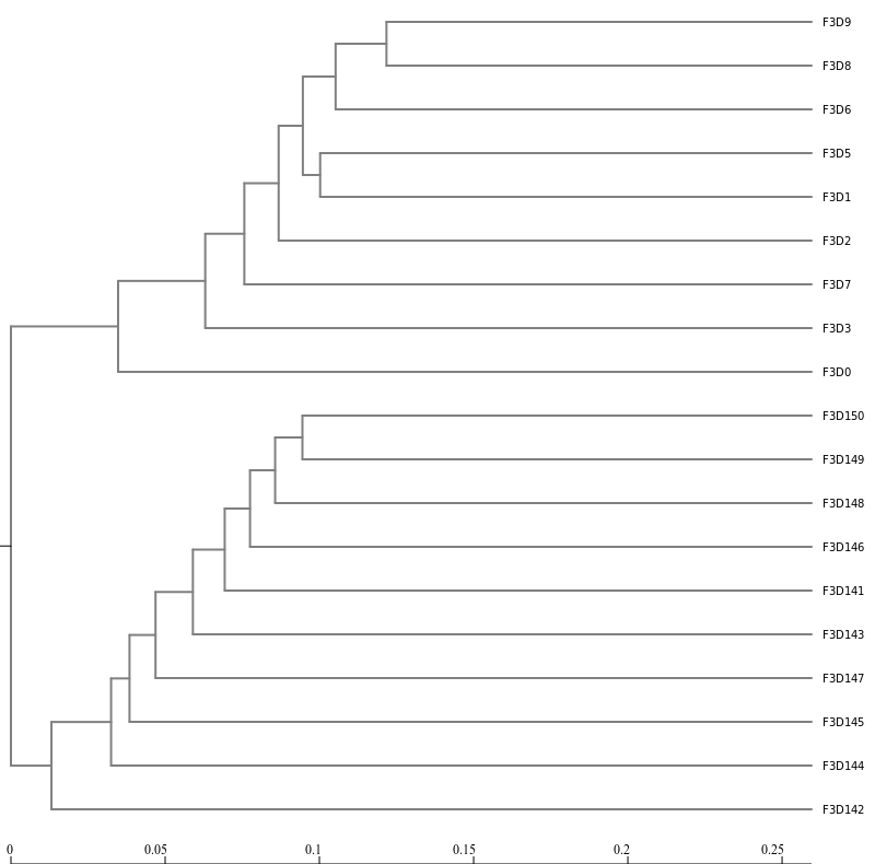
Create pylogenetic tree showing the relatedness of samples (Newick Displaytool)
Click on galaxy-workflows-activityWorkflows in the Galaxy activity bar (on the left side of the screen, or in the top menu bar of older Galaxy instances). You will see a list of all your workflows
Click on galaxy-uploadImport at the top-right of the screen
Paste the following URL into the box labelled “Archived Workflow URL”: https://training.galaxyproject.org/training-material/topics/microbiome/tutorials/mothur-miseq-sop-short/workflows/workflow7_beta_diversity.ga
Click the Import workflow button
Below is a short video demonstrating how to import a workflow from GitHub using this procedure:
Video: Importing a workflow from URL
Run Workflow 7: Beta Diversityworkflow using the following parameters:
“Send results to a new history”: No
param-file“1: Shared File”: the Shared file output from Make.sharedtool
param-collection“2: Subsample shared”: the shared output from Sub.sampletool
Click on Workflows on the Activity Bar on the left.
At the top of the resulting page you will have the option to switch between the My workflows, Workflows shared with me and Public workflows tabs.
Select the tab you want to see all workflows in that category
Search for your desired workflow.
Click on the workflow name: a pop-up window opens with a preview of the workflow.
To run it directly: click Run (top-right).
Recommended: click Import (left of Run) to make your own local copy under Workflows / My Workflows.
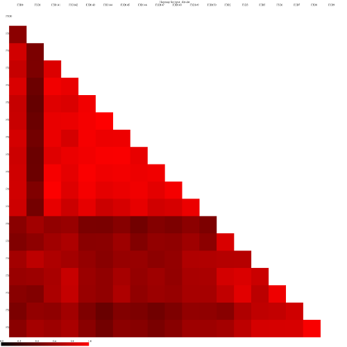
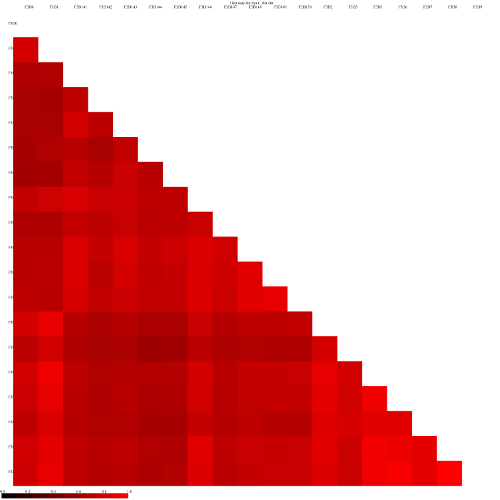
Look at some of the resulting heatmaps (you may have to download the SVG images first). In all of these
heatmaps the red colors indicate communities that are more similar than those with black colors.
For example this is the heatmap for the thetayc calculator (output thetayc.0.03.lt.ave):
and the jclass calulator (output jclass.0.03.lt.ave):
Examine the Venn diagram:
This shows that there were a total of 180 OTUs observed between the 4 time points. Only 76 of those OTUs were
shared by all four time points. We could look deeper at the shared file to see whether those OTUs were
numerically rare or just had a low incidence.
Inspection of the the tree shows that the early and late communities cluster with themselves to the exclusion
of the others.
thetayc.0.03.lt.ave:
jclass.0.03.lt.ave:
Visualisations
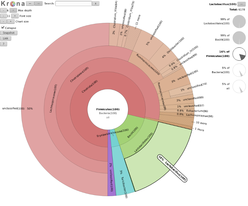
Krona
A tool we can use to visualize the composition of our community, is Krona
Hands On: Krona
First we convert our mothur taxonomy file to a format compatible with Krona
Taxonomy-to-Krona ( Galaxy version 1.0) with the following parameters
param-collection“Taxonomy file”: the taxonomy output from Classify.otu
Krona pie chart ( Galaxy version 2.7.1+galaxy0) with the following parameters
“Type of input”: Tabular
param-collection“Input file”: the taxonomy output from Taxonomy-to-Kronatool
The resulting file is an HTML file containing an interactive visualization. For instance try double-clicking the
innermost ring labeled “Bacteroidetes” below:
Question
What percentage of your sample was labelled Lactobacillus?
Explore the Krona plot, double click on Firmicutes, here you should see Lactobacillus
clearly (16% in our case), click on this segment and the right-hand side will show you the percentages at
any point in the hierarchy (here 5% of all)
You may have noticed that this plot shows the results for all samples together. In many
cases however, you would like to be able to compare results for different samples.
In order to save computation time, mothur pools all reads into a single file, and uses
the count table file to keep track of which samples the reads came from. However, Krona
does not understand the mothur count table format, so we cannot use that to supply information
about the groups. But luckily we can get Classify.otutool to output per-sample
taxonomy files. In the following exercise, we will create a Krona plot with per-sample subplots.
Question: Exercise: per-sample plots
Try to create per-sample Krona plots. An few hints are given below, and the full answer
is given in the solution box.
Re-run galaxy-refresh the Classify.otutool tool we ran earlier
See if you can find a parameter to output a taxonomy file per sample (group)
Run Taxonomy-to-Kronatool again on the per-sample taxonomy files (collection)
Run Kronatool
Find the previous run of Classify.otutool in your history
Hit the rerun button galaxy-refresh to load the parameters you used before:
param-file“list”: the list output from Cluster.splittool
param-file“count”: the count table from Remove.groupstool
param-file“taxonomy”: the taxonomy output from Remove.groupstool
“label”: 0.03
Add new parameter setting:
“persample - allows you to find a consensus taxonomy for each group”: Yes
You should now have a collection with per-sample files
Taxonomy-to-Krona ( Galaxy version 1.0) with the following parameters
param-collection“Taxonomy file”: the taxonomy collection from Classify.otutool
Krona pie chart ( Galaxy version 2.7.1+galaxy0) with the following parameters
“Type of input”: Tabular
param-collection“Input file”: the collection from Taxonomy-to-Kronatool
“Combine data from multiple datasets?”: No
The final result should look something like this (switch between samples via the list on the left):
Further information, including links to documentation and original publications, regarding the tools, analysis techniques and the interpretation of results described in this tutorial can be found here.
References
DeSantis, T. Z., P. Hugenholtz, N. Larsen, M. Rojas, E. L. Brodie et al., 2006 Greengenes, a Chimera-Checked 16S rRNA Gene Database and Workbench Compatible with ARB. Applied and Environmental Microbiology 72: 5069–5072. 10.1128/aem.03006-05
Liu, Z., T. Z. DeSantis, G. L. Andersen, and R. Knight, 2008 Accurate taxonomy assignments from 16S rRNA sequences produced by highly parallel pyrosequencers. Nucleic Acids Research 36: e120–e120. 10.1093/nar/gkn491
Schloss, P. D., S. L. Westcott, T. Ryabin, J. R. Hall, M. Hartmann et al., 2009 Introducing mothur: open-source, platform-independent, community-supported software for describing and comparing microbial communities. Appl. Environ. Microbiol. 75: 7537–7541.
Wooley, J. C., A. Godzik, and I. Friedberg, 2010 A Primer on Metagenomics (P. E. Bourne, Ed.). PLoS Computational Biology 6: e1000667. 10.1371/journal.pcbi.1000667
Federhen, S., 2011 The NCBI Taxonomy database. Nucleic Acids Research 40: D136–D143. 10.1093/nar/gkr1178
Bonilla-Rosso, G., L. E. Eguiarte, D. Romero, M. Travisano, and V. Souza, 2012 Understanding microbial community diversity metrics derived from metagenomes: performance evaluation using simulated data sets. FEMS Microbiology Ecology 82: 37–49. 10.1111/j.1574-6941.2012.01405.x
Quast, C., E. Pruesse, P. Yilmaz, J. Gerken, T. Schweer et al., 2012 The SILVA ribosomal RNA gene database project: improved data processing and web-based tools. Nucleic Acids Research 41: D590–D596. 10.1093/nar/gks1219
Schloss, P. D., 2012 Secondary structure improves OTU assignments of 16S rRNA gene sequences. The ISME Journal 7: 457–460. 10.1038/ismej.2012.102
Cole, J. R., Q. Wang, J. A. Fish, B. Chai, D. M. McGarrell et al., 2013 Ribosomal Database Project: data and tools for high throughput rRNA analysis. Nucleic Acids Research 42: D633–D642. 10.1093/nar/gkt1244
Finotello, F., E. Mastrorilli, and B. D. Camillo, 2016 Measuring the diversity of the human microbiota with targeted next-generation sequencing. Briefings in Bioinformatics bbw119. 10.1093/bib/bbw119
Fouhy, F., A. G. Clooney, C. Stanton, M. J. Claesson, and P. D. Cotter, 2016 16S rRNA gene sequencing of mock microbial populations- impact of DNA extraction method, primer choice and sequencing platform. BMC Microbiology 16: 10.1186/s12866-016-0738-z
Rognes, T., T. Flouri, B. Nichols, C. Quince, and F. Mahé, 2016 VSEARCH: a versatile open source tool for metagenomics. PeerJ 4: e2584. 10.7717/peerj.2584
Singer, E., B. Andreopoulos, R. M. Bowers, J. Lee, S. Deshpande et al., 2016 Next generation sequencing data of a defined microbial mock community. Scientific Data 3: 160081. 10.1038/sdata.2016.81
Balvočiūtė, M., and D. H. Huson, 2017 SILVA, RDP, Greengenes, NCBI and OTT — how do these taxonomies compare? BMC Genomics 18: 10.1186/s12864-017-3501-4
Feedback
Did you use this material as an instructor? Feel free to give us feedback on how it went.
Did you use this material as a learner or student? Click the form below to leave feedback.
Hiltemann, Saskia, Rasche, Helena et al., 2023 Galaxy Training: A Powerful Framework for Teaching! PLOS Computational Biology 10.1371/journal.pcbi.1010752
Batut et al., 2018 Community-Driven Data Analysis Training for Biology Cell Systems 10.1016/j.cels.2018.05.012
@misc{microbiome-mothur-miseq-sop-short,
author = "Saskia Hiltemann and Bérénice Batut and Dave Clements",
	title = "16S Microbial Analysis with mothur (short) (Galaxy Training Materials)",
	year = "",
	month = "",
	day = "",
	url = "\url{https://training.galaxyproject.org/training-material/topics/microbiome/tutorials/mothur-miseq-sop-short/tutorial.html}",
	note = "[Online; accessed TODAY]"
}
@article{Hiltemann_2023,
	doi = {10.1371/journal.pcbi.1010752},
	url = {https://doi.org/10.1371%2Fjournal.pcbi.1010752},
	year = 2023,
	month = {jan},
	publisher = {Public Library of Science ({PLoS})},
	volume = {19},
	number = {1},
	pages = {e1010752},
	author = {Saskia Hiltemann and Helena Rasche and Simon Gladman and Hans-Rudolf Hotz and Delphine Larivi{\`{e}}re and Daniel Blankenberg and Pratik D. Jagtap and Thomas Wollmann and Anthony Bretaudeau and Nadia Gou{\'{e}} and Timothy J. Griffin and Coline Royaux and Yvan Le Bras and Subina Mehta and Anna Syme and Frederik Coppens and Bert Droesbeke and Nicola Soranzo and Wendi Bacon and Fotis Psomopoulos and Crist{\'{o}}bal Gallardo-Alba and John Davis and Melanie Christine Föll and Matthias Fahrner and Maria A. Doyle and Beatriz Serrano-Solano and Anne Claire Fouilloux and Peter van Heusden and Wolfgang Maier and Dave Clements and Florian Heyl and Björn Grüning and B{\'{e}}r{\'{e}}nice Batut and},
	editor = {Francis Ouellette},
	title = {Galaxy Training: A powerful framework for teaching!},
	journal = {PLoS Comput Biol}
}
Funding
These individuals or organisations provided funding support for the development of this resource
3 stars:
Liked: the details are good
Disliked: many many of the things are different when you work your own samples, i had to modify many of the parameters but thats fine but, there were many errors in workflows, my workflow 5 didnt ran, it required mock file in remove. lineage, but the when you are working on samples other than galaxy there is no mock samples file, further the workflow 6 and work flow 7 also didnt ran, the sub.samples step is not clearly mentioned before the workflow 7 and if i run the sub.samples tool seperately tw it do not gives the shared file, which is required.
May 2023
5 stars:
Liked: A really comprehensive breakdown of how to do this analysis. All the steps of the analysis were well laid out in a good amount of detail that if you followed closely you should be equipped with the tools to run the same analysis yourself. The instructor was excellent and covered a lot of material, maintaining good clarity throughout.
Disliked: I don't think anything could be improved upon. It is a long tutorial but the length of the tutorial is necessary to cover the content in a thorough way, as was done. Thank you.
March 2022
4 stars:
Liked: I WAS NOT AWARE THE OPTION WHERE YOU CAN GROUP YOUR DATA AND ANALYZE IT AS A COLLECTION, THANKS A LOT
5 stars:
Liked: the pace and amount of information was just right, very clear and understandable :)
5 stars:
Disliked: great tutorial, very well explained
December 2021
5 stars:
Liked: Stepwise, just in time learning and great links to additional information
Disliked: (Having the video helped), but the steps were all included.
August 2019
4 stars:
Disliked: The Krona plot - this appears to be of all samples. Would be good to per sample. Might not be possible with Phinch. As for Phinch, that is no longer web accessible but standalone and has dropped functionality.
Questions:


(slide credit: http://slideplayer.com/slide/4559004/ )
 Guerrero Negro mat, (b) Human gut and (c) Mouse gut, using a range of different methods (separate subpanels within each group). The x-axis of each graph shows region sequenced. The y-axis shows abundance as a fraction of the total number of sequences in the community. The legend shows colors for phyla (consistent across graphs).")
Open image in new tab