A diversity index is a quantitative measure that is used to assess the level of diversity or variety within a particular system, such as a biological community, a population, or a workplace. It provides a way to capture and quantify the distribution of different types or categories within a system.
In various fields, diversity indexes are employed to understand and compare the composition and richness of various elements. Apart from ecology, fields such as social and cultural science are interested in the diversity within a population or workplace. In these cases, the indexes may consider factors like age, gender, ethnicity, or other relevant characteristics to assess the diversity and inclusiveness of a group or organization.
To study microbiome data, indirect methods like metagenomics can be used. Metagenomic samples contain DNA from different organisms at a specific site, where the sample was collected. Metagenomic data can be used to find out which organisms coexist in that niche and which genes are present in the different organisms.
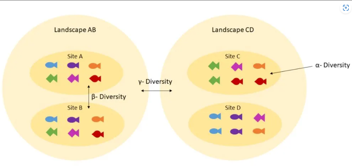
Related to ecology, the term diversity describes the number of different species present in one particular area and their relative abundance. More specifically, several different metrics of diversity can be calculated. The most common ones are \(\alpha\), \(\beta\) and \(\gamma\) diversity:
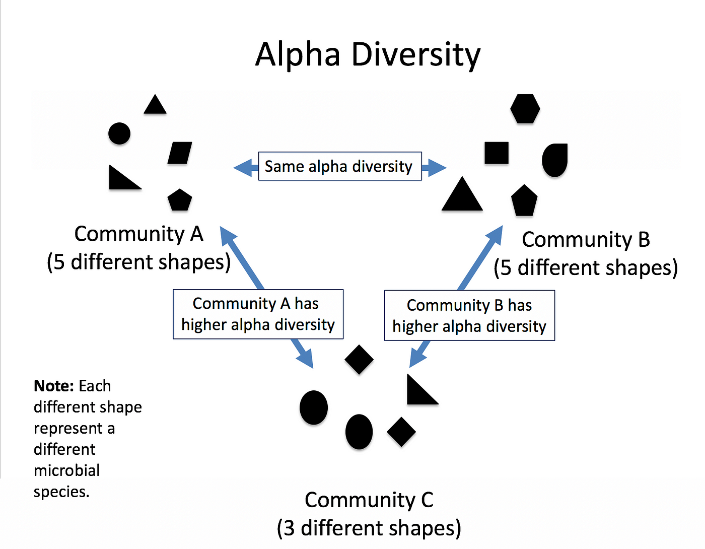
\(\alpha\) diversity describes the diversity within a community
It considers the number of different species in an environment (also referred to as species richness). Additionally, it can take the abundance of each species into account to measure how evenly individuals are distributed across the sample (also referred to as species evenness).
\(\beta\) diversity compare the diversity between different communities by measuring their distance
\(\gamma\) diversity is a measure of the overall diversity for the different ecosystems within a region.
In this analysis we will use Galaxy for calculating different alpha diversity indexes and the Bray-Curtis dissimilarity index for β diversity.
Background on data
The dataset we will use for this tutorial comes from an oasis in the Mexican desert called Cuatro Ciénegas (Okie et al. 2020). The researchers were interested in genomic traits that affect the rates and costs of biochemical information processing within cells. They performed a whole-ecosystem experiment, thus fertilizing the pond to achieve nutrient enriched conditions.
Here we will use 2 datasets:
JP4D: a microbiome sample collected from the Lagunita Fertilized Pond
JC1A: a control samples from a control mesocosm.
The datasets differ in size, but according to the authors this doesn’t matter for their analysis of genomic traits. Also, they underline that differences between the two samples reflect trait-mediated ecological dynamics instead of microevolutionary changes as the duration of the experiment was only 32 days. This means that depending on available nutrients, specific lineages within the pond grow more successfully than others because of their genomic traits. The samples have been analysed as explained in the Taxonomic profiling tutorial.
In a nutshell, taxonomic labels have been assigned to the metagenomics data using Kraken2 to find out which species are present in the samples. Finally, species abundance was estimated using Bracken. For this tutorial, we will use the output file of Bracken.
To get an overview, you can find a Krona chart visualizing the different species present in the two samples.
The dataset we will work with in this tutorial is the output file of Bracken, which estimates species abundance.
name	taxonomy_id	taxonomy_lvl	kraken_assigned_reads	added_reads	new_est_reads	fraction_total_reads
Paracoccus sp. MC1862	2760307	S	98	4	102	0.00169
Paracoccus sp. AK26	2589076	S	85	8	93	0.00154
Paracoccus sp. Arc7-R13	2500532	S	67	13	80	0.00133
Paracoccus sp. BM15	1529068	S	27	1	28	0.00046
Paracoccus sanguinis	1545044	S	142	37	179	0.00297
Paracoccus contaminans	1945662	S	87	18	105	0.00174
Paracoccus aminovorans	34004	S	86	26	112	0.00186
Question
What information do the different columns contain?
species name
taxonomy ID
taxonomic level: K_kingdom, P_phylum, C_class, O_order, F_family, G_genus, and S_species
reads assigned by Kraken
additional reads added by Bracken: In order to estimate species abundance, Bracken reestimates the reads assigned by Kraken using bayesian reestimation. For details on the procedure, have a look into the Bracken publication.
sum of column 4 and column 5
fraction of the reads assigned to the particular species and the total reads
It is possible to calculate \(\alpha\) and \(\beta\) diversity also on other datasets than the Bracken output. Any tool that outputs taxonomy abundances can be used prior to the diversity analysis. To use Krakentools (as described here), the respective output file needs to be converted into the correct table format and filtered for the taxonomic rank “species”. This step is not necessary when using Bracken output as already only the species level is listed.
Any analysis should get its own Galaxy history. So let’s start by creating a new one:
Hands On: Data upload
Create a new history for this analysis
To create a new history simply click the new-history icon at the top of the history panel:
Rename the history
Click on galaxy-pencil (Edit) next to the history name (which by default is “Unnamed history”)
Type the new name
Click on Save
To cancel renaming, click the galaxy-undo “Cancel” button
If you do not have the galaxy-pencil (Edit) next to the history name (which can be the case if you are using an older version of Galaxy) do the following:
Click on Unnamed history (or the current name of the history) (Click to rename history) at the top of your history panel
Type the new name
Press Enter
We need now to import the data
Hands On: Import datasets
Import the following samples via link from Zenodo or Galaxy shared data libraries:
Click galaxy-uploadUpload at the top of the activity panel
Select galaxy-wf-editPaste/Fetch Data
Paste the link(s) into the text field
Press Start
Close the window
As an alternative to uploading the data from a URL or your computer, the files may also have been made available from a shared data library:
Go into Libraries (left panel)
Navigate to the correct folder as indicated by your instructor.
On most Galaxies tutorial data will be provided in a folder named GTN - Material –> Topic Name -> Tutorial Name.
Select the desired files
Click on Add to Historygalaxy-dropdown near the top and select as Datasets from the dropdown menu
In the pop-up window, choose
“Select history”: the history you want to import the data to (or create a new one)
Click on Import
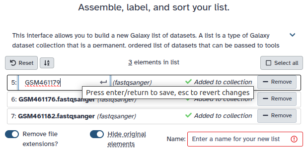
Create a collection.
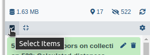
Click on galaxy-selectorSelect Items at the top of the history panel
Check all the datasets in your history you would like to include
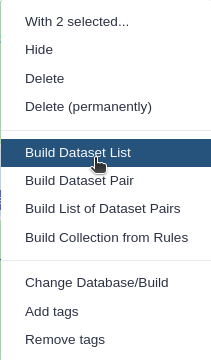
Click n of N selected and choose Advanced Build List
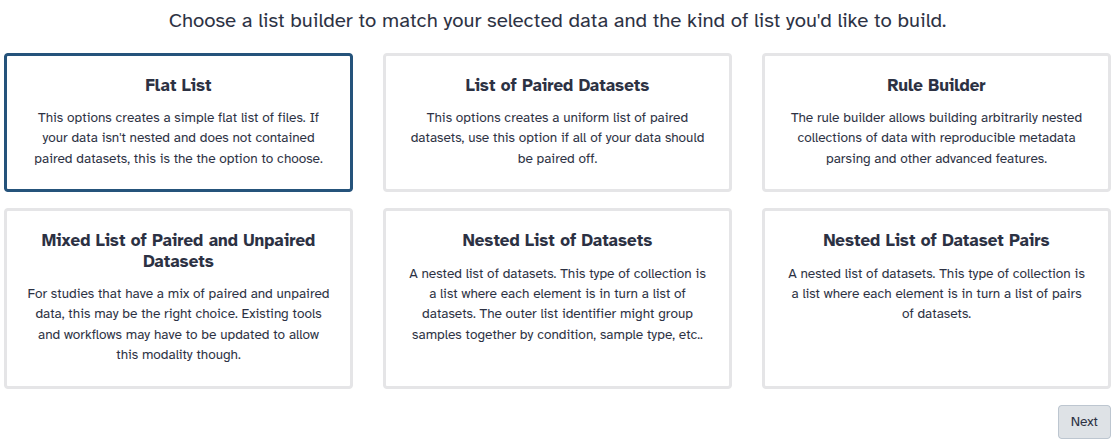
You are in collection building wizard. Choose Flat List and click ‘Next’ button at the right bottom corner.
Double clcik on the file names to edit. For example, remove file extensions or common prefix/suffixes to cleanup the names.
Enter a name for your collection
Click Build to build your collection
Click on the checkmark icon at the top of your history again
Calculating \(\alpha\) diversity
Theory of \(\alpha\) diversity
\(\alpha\) diversity describes the diversity within a community. There are several different indexes used to calculate \(\alpha\) diversity because different indexes capture different aspects of diversity and have varying sensitivities to different factors. These indexes have been developed to address specific research questions, account for different ecological or population characteristics, or highlight certain aspects of diversity.
Metrics of \(\alpha\) diversity can be grouped into different classes:
Richness estimates the quantity of distinct species within a sample
Margalef’s richness indicates the estimated species richness, accounting for the community size. This metric takes into account that a larger community size can support a greater number of species (Margalef 1969)
\[D = \frac{(S - 1)}{\log(n)}\]
With
\(S\) the total number of species,
\(n\) the total number of individuals in the sample
Chao1 estimates the true species richness or diversity of a community, particularly when there might be rare or unobserved species. Chao1 estimates the number of unobserved species based on the number of singletons and doubletons. It assumes that there are additional rare species that are likely to exist but have not been observed. The estimation considers the number of unobserved singletons and doubletons and incorporates them into the observed species richness to provide an estimate of the true species richness (Chao and Lee 1992).
\(n_{1}\) the number of species represented by a single individual (singletons),
\(n_{2}\) the number of species represented by two individuals (doubletons).
ACE (Abundance-based Coverage Estimator) takes into account the abundance distribution of observed species and incorporates the presence of rare or unobserved species. ACE estimates the number of unobserved species based on the abundance distribution and incorporates it into the observed species richness. It takes into account the relative rarity of observed species and uses this information to estimate the true species richness.
Evenness evaluates the relative abundances of species rather than their total count
Pielou’s evenness quantifies how close the community’s diversity is to the maximum possible diversity. This index is calculated by taking the Shannon Diversity Index (which measures the overall diversity of the community) and dividing it by the maximum possible diversity given the observed species richness (Pielou 1966).
\[J = \frac{H'}{ln(S)}\]
With:
\(H'\) the Shannon Weiner diversity Index
\(S\) the total number of species in a sample, across all samples in dataset.
Diversity incorporates both the relative abundances and total count of distinct species
Shannons index calculates the uncertainty in predicting the species identity of an individual that is selected from a community (Shannon 1948).
\[H' = - \sum_{i=1}^{S} p_i \ln (p_i)\]
With \(p_i\) the proportion of individuals of species \(i\)
The index ranges from 0 to a maximum value that depends on the number of species and their relative abundances. The higher the Shannon index value, the greater the diversity within the community.
Berger-Parker index expresses the proportional importance of the most abundant type. This index is highly biased by sample size and richness (Berger and Parker 1970 ).
\[D = \frac{n_{max}}{N}\]
With:
\(n_{max}\) the abundance of the most dominant species
\(N\) the total number of individuals (sum of all abundances)
In contrast to the Shannon index, which considers both species richness and evenness, the Berger-Parker index emphasizes the dominance of a particular species.
Simpsons index calculates the probability that two individuals selected from a community will be of the same species. Small values are observed in datasets of high diversity and large values in datasets of low diversity (SIMPSON 1949).
\(n_i\) the number of individuals in species \(i\)
\(N\) total number of individuals of all species
\(\frac{n_i}{N} = p_i\) the proportion of individuals of species \(i\)
\(S\) the species richness.
The index ranges from 0 to 1, with 1 representing maximum diversity. A value of 0.6 indicates that two randomly selected individuals from the community have 60% probability to belong to different species.
Inverse Simpons index is the transformation of Simpsons index that increases with increasing diversity. A higher Inverse Simpson’s index value signifies a community with a greater number of species and a more even distribution of individuals among those species. The index ranges from 1 to the total number of species in the community, with higher values indicating higher diversity.
Fishers alpha index describes the relationship between the number of species and the number of individuals in those species. Parametric index of diversity that assumes that the abundance of species follows a logarithmic series distribution (Fisher et al. 1943).
\[S = a \cdot \ln \left(1+\frac{n}{a}\right)\]
With:
\(S\) the number of taxa
\(n\) the number of individuals
\(a\) the the Fisher’s alpha.
A higher Fisher’s alpha value indicates greater species diversity within the sampled area.
Computing α diversity using Galaxy
KrakenTools is a suite of scripts designed to help Kraken users with downstream analysis of Kraken results. The Krakentool Calculate alpha diversity offers the possibility to calculate five different \(\alpha\) diversity indexes:
Shannon’s \(\alpha\) diversity
Berger Parker’s \(\alpha\)
Simpson’s diversity
Inverse Simpson’s diversity
Fisher’s index
Hands On: Calculate α diversity with Krakentools
Krakentools: Calculate alpha diversity ( Galaxy version 1.2+galaxy1) with the following parameters:
Run Krakentools: Calculate alpha diversity ( Galaxy version 1.2+galaxy1) with the 4 other indexes
Question
What are the values of 5 different \(\alpha\) indexes?
How should we interpret the different \(\alpha\) indexes?
Are the results consistent among the different indexes?
What is the dominant species in the samples? What is the problem we can see?
The results of five \(\alpha\) indexes for both the JC1A and JP4D sample as well as an explanation of the meaning of these values.
JC1A
JP4D
Shannon
2.06
3.74
Berger-Parker
0.46
0.08
Simpson
0.74
0.97
Inverse Simpson
3.92
28.84
Fisher
209.73
456.61
Intepretation of the different indexes:
Shannon index: the index ranges from 0 to a maximum value that depends on the number of species and their relative abundances. The higher the Shannon index value, the greater the diversity within the community. A value of ~4 indicates a relatively high level of diversity within the community.
Berger-Parker index: In contrast to the Shannon index, which considers both species richness and evenness, the Berger-Parker index emphasizes the dominance of a particular species.
For JC1A, a value of 0.46 suggests that a single species dominates the community, as it represents 46% of the total individuals in the community. This indicates a relatively low level of species evenness, meaning that the abundance of individuals is heavily skewed towards one dominant species. A value of 0.46 indicates that the community is heavily influenced by one species, while the other species in the community are less abundant.
In the case of JP4D, the dominant species accounts for only 8 % of the total individuals, which implies a more balanced distribution of individuals among different species compared to a higher Berger-Parker index value.
Simpson’s index: The index ranges from 0 to 1, with 1 representing maximum diversity. Therefore, value of 0.97 indicates a high level of species diversity and evenness within the community: community is highly diverse, with a relatively even distribution of individuals among different species. In other words, the value of 0.97 indicates that two randomly selected individuals from the community have 97% probability to belong to different species. This implies a rich and balanced community where multiple species coexist in relatively equal abundance.
Inverse Simpson’s index: The Inverse Simpson’s index is the reciprocal of the Simpson’s index, which quantifies species diversity and evenness within a community. A higher Inverse Simpson’s index value signifies a community with a greater number of species and a more even distribution of individuals among those species. The index ranges from 1 to the total number of species in the community, with higher values indicating higher diversity. A value of 3.92 suggests a relatively low level of species diversity within the community and a value of 28.84 suggests a relatively high level of species diversity within the community.
Index
JC1A
JP4D
Shannon
Less diversity as in JP4D
Relatively high level of diversity
Berger-Parker
A single species dominates the community
mMre balanced distribution of individuals among different species
Simpson
Lower level of species diversity and evenness
High level of species diversity and evenness
Inverse Simpson
Relatively low level of species diversity
Relatively high level of species diversity
Fisher
Lower species diversity
Greater species diversity
The results are consistent as all indexes show JP4D to be the more diverse sample compared to JC1A.
When looking at the Bracken files, we see that the dominant species in this samples is Homo sapiens - so us! This should not be part of the samples and is probably due to contamination. This finding should be used to reanalyze the samples and remove the human contamination. For the sake of simplicity we will continue with the samples as is and assume the Homo sapiens to be a species in out samples.
Comment
Apart from Krakentools, there are at least two more tools available in Galaxy that can be used to calculate diversity indexes,
QIIME 2 (Quantitative Insights Into Microbial Ecology 2) is a powerful open-source bioinformatics software package that provides a comprehensive suite of tools and methods for processing, analyzing, and visualizing microbiome data. It offers a modular approach to microbiome analysis, allowing researchers to build flexible analysis pipelines tailored to their specific research goals. The software supports a wide range of data types, including 16S rRNA gene sequencing, metagenomics, metatranscriptomics, and others.
Some of the key features and functionalities of QIIME 2 include:
Diversity Analysis: QIIME 2 allows users to explore and quantify microbial diversity within and between samples. It provides metrics for alpha diversity (within-sample diversity) and beta diversity (between-sample diversity).
The vegan package is a community ecology package in the R programming language. It provides a wide range of tools and methods for analyzing and interpreting ecological data, particularly in the context of community ecology. The package is designed to handle multivariate data and offers various statistical techniques for studying species composition, diversity, and community dynamics.
The vegan package encompasses several functionalities, including:
Diversity Analysis: vegan offers numerous diversity indices, such as species richness, Shannon diversity index, Simpson index, and many others. These indices allow researchers to quantify the diversity of species within a community and compare diversity between different samples or groups.
Ordination Techniques
Community Classification:
Ecological Network Analysis
Ecological Indices
Plotting and Visualization
Calculating \(\beta\) diversity
Theory of \(\beta\) diversity
\(\beta\) diversity measures the distance between two or more separate entities. It therefore describes the difference between two communities or ecosystems.
There are multiple indexes used to calculate \(\beta\) diversity because different indexes emphasize different aspects of compositional dissimilarity between communities or sites.
These indexes have been developed to address specific research questions, accommodate different data types, or provide insights into different dimensions of \(\beta\) diversity.
Jaccard Index measures the proportion of shared species between two samples (Jaccard 1912).
\[J(X, Y) = \frac{\| X ∩ Y\|}{\| X ∪ Y\|}\]
With:
\(X ∩ Y\) the intersection of sets \(X\) and \(Y\), i.e. elements common to both sets
\(X ∪ Y\) the union of sets \(X\) and \(Y\), i.e. all unique elements from both sets combined
Sørensen Index is similar to Jaccard Index, but accounts for species abundance (Sørensen 1948).
\[DSC = \frac{2\| X ∩ Y\|}{\| X\|} + \| Y\|\]
With:
\(X ∩ Y\) the intersection of sets \(X\) and \(Y\), i.e.elements common to both sets
\(\| X\|\) and \(\| Y \|\) the cardinalities of the two sets, i.e. the number of elements in each set.
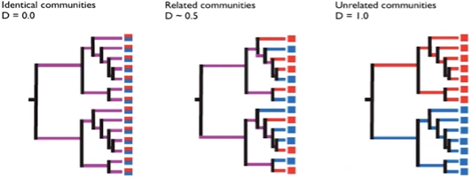
Bray-Curtis Dissimilarity measures the dissimilarity of species abundances between two samples (Bray and Curtis 1957).
\[BC_{ij} = 1 - \frac{2C_{ij}}{S_{i} + S_{j}}\]
With:
\(C_{ij}\) the sum of the absolute differences in abundances between corresponding species in samples \(i\) and \(j\)
\(S_{i}\) the total abundance or sum of species abundances in sample \(i\)
\(S_{j}\) the total abundance or sum of species abundances in sample \(j\)
The higher the dissimilarity value, the greater the difference in species composition or abundances.
Kulczynski Dissimilarity masures the dissimilarity in the proportional abundances of shared species.
\(S_{AB}\) the number of shared species between communities \(A\) and \(B\)
\(S_{A}\) the number of species in community \(A\)
\(S_{B}\) the number of species in community \(B\)
UniFrac incorporates information on phylogenetic distances between observed species in the computation. Can be calculated either weighted (accounts for abundances) or unweighted (accounts only for richness).
Computing \(\beta\) diversity using Galaxy
Hands On: Calculate β diversity with Krakentools
Krakentools: Calculate beta diversity (Bray-Curtis dissimilarity) ( Galaxy version 1.2+galaxy1) with the following parameters:
“Specify type of input file”: Bracken species abundance file
Question
What is the Bray-Curtis dissimilarity calculated for the two samples?
How can we interpret Bray-Curtis dissimilarity between the two samples?
The output file gives you a table comparing sample 0 and 1, respectively. Consequently, comparing 0 to 0 and 1 to 1 results in a dissimilarity of 0, as those are exactly the same. Comparing sample 0 to sample 1 shows a Bray-Curtis dissimilarity of 0.701.
The Bray-Curtis dissimilarity measures the dissimiliraty of two samples. Consequently, an output of 0 represents two samples that are exactly the same, while an output of 1 means they are maximally divergent. In our case, a Bray-Curtis dissimilarity of 0.7 suggests that there is a substantial difference in the species composition or abundances between the two communities being compared. The higher the dissimilarity value, the greater the difference in species composition or abundances.
Evaluation of different diversity metrics
Bonilla-Rosso et al. did performance evaluation of different diversity metrics using simulated data sets Bonilla-Rosso et al. 2012. However, it is important to note that none of the estimated metrics showed statistical similarity to their corresponding parameters in the source communities. Moreover, the results obtained were inconsistent across the samples.
This inconsistency can be attributed to the fact that individual metrics only provide a specific perspective on diversity and are prone to bias in their estimation, leading to incorrect ranking of the samples.
In summary, relying solely on single-diversity metrics may not be enough to accurately compare the diversity between two communities. Instead, we recommend utilizing multi-dimensional metrics to capture diverse rankings across different scales of diversity, which can be affected differently in manipulative studies.
Multidimensional diversity metrics, also known as multivariate diversity metrics, are quantitative measures that capture multiple dimensions or aspects of diversity simultaneously. These metrics go beyond single-diversity metrics, such as species richness or Shannon entropy, which provide a one-dimensional representation of diversity.
In contrast, multidimensional diversity metrics take into account various attributes or characteristics of species or communities to provide a more comprehensive understanding of diversity. These attributes can include species abundances, functional traits, phylogenetic relationships, or spatial distributions.
The choice and composition of dimensions in multidimensional diversity metrics depend on the research context and the specific objectives of the study. Some aspects, multidimensional diversity metrics take into account, include:
Functional Diversity: This metric considers the range and variation of functional traits among species within a community. It assesses the diversity of ecological roles and functional strategies present, contributing to ecosystem functioning and resilience.
Phylogenetic Diversity: This metric incorporates the evolutionary relationships among species within a community. It quantifies the diversity based on the length and topology of the phylogenetic tree, highlighting the evolutionary history and relatedness of species.
Spatial Diversity: This metric incorporates spatial patterns and distributions of species within a landscape or ecosystem. It considers the heterogeneity of habitats, connectivity, and the arrangement of species populations across space.
Multidimensional diversity metrics offer a more nuanced and holistic perspective on biodiversity, capturing different facets and dimensions of ecological variation. They provide insights into the ecological processes shaping communities and ecosystems and can be valuable in conservation planning, ecosystem management, and understanding the functional implications of biodiversity patterns.
Expressing the compositional complexity of an assemblage cannot be accomplished with a single numerical value. Traditional measures like diversities (Hill numbers) and entropies (Rényi entropies) vary in their order \(q\), which determines the extent to which rare or common species are emphasized. The ranking and comparison of assemblages rely on the chosen value of \(q\).
Instead of selecting a few measures to describe an assemblage, it is preferable to present a continuous profile that depicts diversity or entropy as a function of \(q\) (where \(q \sep 0\)). This approach enables a visual comparison of the compositional complexities among multiple assemblages and facilitates the assessment of the evenness in the relative abundance distributions of the assemblages. In practice, the profile is typically plotted for values of \(q\) ranging from 0 to \(q =\) 3 or 4, beyond which there is usually little change.
Hill numbers, also known as diversity indices or diversity measures, are mathematical metrics used to quantify the diversity or richness of a biological community. They were developed by ecologist Robert H. Whittaker and are widely used in ecology and biodiversity studies.
Hill numbers provide a way to summarize and compare the diversity of different communities based on the abundance or occurrence of different species within those communities. These numbers take into account both the number of species present and their relative abundances. The higher the Hill number, the greater the diversity or richness of the community.
Hill numbers are often represented by the symbol \(D\), followed by a subscript that indicates the order of diversity. The order of diversity determines the weight given to rare versus common species. Commonly used Hill numbers include:
Species richness (\(D\_0\)): This is the simplest Hill number and represents the total number of species in a community, without considering their abundances. It provides a basic measure of biodiversity based on species count.
Shannon diversity index (\(D\_1\)): This index incorporates both species richness and evenness. It takes into account both the number of species and their relative abundances, providing a more comprehensive measure of diversity.
Simpson diversity index (\(D\_2\)): This index focuses on the dominance or concentration of species within a community. It considers both species richness and the probability that two individuals randomly selected from the community belong to the same species.
Rényi entropy
Rényi entropy is a concept in information theory and statistical physics introduced by Alfréd Rényi, a Hungarian mathematician. It is a generalization of the Shannon entropy, which measures the uncertainty or information content of a random variable or probability distribution.
The Rényi entropy of a discrete probability distribution is defined by the parameter \(\alpha\), which determines the order of the entropy. The formula for calculating Rényi entropy is:
where \(P = {p\_1, p\_2, ..., p\_N}\) is the probability distribution of \(N\) discrete events or states, and \(p\_i\) represents the probability of the ith event.
The value of \(\alpha\) determines the properties of Rényi entropy. When \(\alpha = 1\), Rényi entropy reduces to Shannon entropy, providing a measure of average uncertainty or information content. As \(\alpha\) approaches 0, Rényi entropy converges to the minimum value, representing the most certain or least diverse distribution. Conversely, as \(\alpha\) approaches infinity, Rényi entropy approaches the maximum value, indicating a uniform or maximally diverse distribution.
Rényi entropy has applications in various fields, including information theory, statistical physics, and data analysis. It offers a way to quantify the diversity or randomness of a system beyond the traditional Shannon entropy, allowing for a more nuanced understanding of information content and structure.
For further information on how to choose the best diversity metric also check:
In this tutorial, we look how to calculate \(\alpha\) and \(\beta\) diversity from microbiome data. We apply Krakentools to calculate the \(\alpha\) and \(\beta\) diversity of two microbiome sample datasets.
You've Finished the Tutorial
Please also consider filling out the Feedback Form as well!
Key points
There are 2 different types of diversity metrics (α and β diversity)
Krakentools can be used in Galaxy for calculating the diversity
Frequently Asked Questions
Have questions about this tutorial? Have a look at the available FAQ pages and support channels
Further information, including links to documentation and original publications, regarding the tools, analysis techniques and the interpretation of results described in this tutorial can be found here.
Fisher, R. A., A. S. Corbet, and C. B. Williams, 1943 The Relation Between the Number of Species and the Number of Individuals in a Random Sample of an Animal Population. The Journal of Animal Ecology 12: 42. 10.2307/1411
Shannon, C. E., 1948 A Mathematical Theory of Communication. Bell System Technical Journal 27: 379–423. 10.1002/j.1538-7305.1948.tb01338.x
Sørensen, T., 1948 A method of establishing groups of equal amplitude in plant sociology based on similarity of species and its application to analyses of the vegetation on Danish commons. Kongelige Danske Videnskabernes Selskab. 1–34.
SIMPSON, E. H., 1949 Measurement of Diversity. Nature 163: 688. 10.1038/163688a0
Bray, J. R., and J. T. Curtis, 1957 An Ordination of the Upland Forest Communities of Southern Wisconsin. Ecological Monographs 27: 325–349. 10.2307/1942268
Pielou, E. C., 1966 The measurement of diversity in different types of biological collections. Journal of Theoretical Biology 13: 131–144. 10.1016/0022-5193(66)90013-0
Margalef, R., 1969 Perspectives in Ecological Theory. Oikos 20: 571. 10.2307/3543237
Berger, W. H., and F. L. Parker, 1970 Diversity of planktonic foraminifera in deep-sea sediments. Science (New York, N.Y.) 168: 1345–1347. 10.1126/science.168.3937.1345.
Chao, A., and S.-M. Lee, 1992 Estimating the Number of Classes via Sample Coverage. Journal of the American Statistical Association 87: 210–217. 10.1080/01621459.1992.10475194
Bonilla-Rosso, G., L. E. Eguiarte, D. Romero, M. Travisano, and V. Souza, 2012 Understanding microbial community diversity metrics derived from metagenomes: performance evaluation using simulated data sets. FEMS microbiology ecology 82: 37–49. 10.1111/j.1574-6941.2012.01405.x
Finotello, F., E. Mastrorilli, and B. Di Camillo, 2018 Measuring the diversity of the human microbiota with targeted next-generation sequencing. Briefings in bioinformatics 19: 679–692. 10.1093/bib/bbw119
Bolyen, E., J. R. Rideout, M. R. Dillon, N. A. Bokulich, C. C. Abnet et al., 2019 Reproducible, interactive, scalable and extensible microbiome data science using QIIME 2. Nature biotechnology 37: 852–857. 10.1038/s41587-019-0209-9
Okie, J. G., A. T. Poret-Peterson, Z. M. Lee, A. Richter, L. D. Alcaraz et al., 2020 Genomic adaptations in information processing underpin trophic strategy in a whole-ecosystem nutrient enrichment experiment. eLife 9: 10.7554/eLife.49816
Feedback
Did you use this material as an instructor? Feel free to give us feedback on how it went.
Did you use this material as a learner or student? Click the form below to leave feedback.
Hiltemann, Saskia, Rasche, Helena et al., 2023 Galaxy Training: A Powerful Framework for Teaching! PLOS Computational Biology 10.1371/journal.pcbi.1010752
Batut et al., 2018 Community-Driven Data Analysis Training for Biology Cell Systems 10.1016/j.cels.2018.05.012
@misc{microbiome-diversity,
author = "Sophia Hampe and Bérénice Batut and Paul Zierep",
	title = "Calculating α and β diversity from microbiome taxonomic data (Galaxy Training Materials)",
	year = "",
	month = "",
	day = "",
	url = "\url{https://training.galaxyproject.org/training-material/topics/microbiome/tutorials/diversity/tutorial.html}",
	note = "[Online; accessed TODAY]"
}
@article{Hiltemann_2023,
	doi = {10.1371/journal.pcbi.1010752},
	url = {https://doi.org/10.1371%2Fjournal.pcbi.1010752},
	year = 2023,
	month = {jan},
	publisher = {Public Library of Science ({PLoS})},
	volume = {19},
	number = {1},
	pages = {e1010752},
	author = {Saskia Hiltemann and Helena Rasche and Simon Gladman and Hans-Rudolf Hotz and Delphine Larivi{\`{e}}re and Daniel Blankenberg and Pratik D. Jagtap and Thomas Wollmann and Anthony Bretaudeau and Nadia Gou{\'{e}} and Timothy J. Griffin and Coline Royaux and Yvan Le Bras and Subina Mehta and Anna Syme and Frederik Coppens and Bert Droesbeke and Nicola Soranzo and Wendi Bacon and Fotis Psomopoulos and Crist{\'{o}}bal Gallardo-Alba and John Davis and Melanie Christine Föll and Matthias Fahrner and Maria A. Doyle and Beatriz Serrano-Solano and Anne Claire Fouilloux and Peter van Heusden and Wolfgang Maier and Dave Clements and Florian Heyl and Björn Grüning and B{\'{e}}r{\'{e}}nice Batut and},
	editor = {Francis Ouellette},
	title = {Galaxy Training: A powerful framework for teaching!},
	journal = {PLoS Comput Biol}
}
Congratulations on successfully completing this tutorial!
You can use Ephemeris's shed-tools install command to install the tools used in this tutorial.
5 stars:
Liked: I enjoyed the basics. That means it really nice to read what are the differences in diversity and how they are calculated.
Disliked: not sure.
January 2025
5 stars:
Liked: SIMPLE
Disliked: New method
October 2024
5 stars:
Liked: the flow of the tutorial is well organised
Questions:


 (Source: Pedro J Torres)
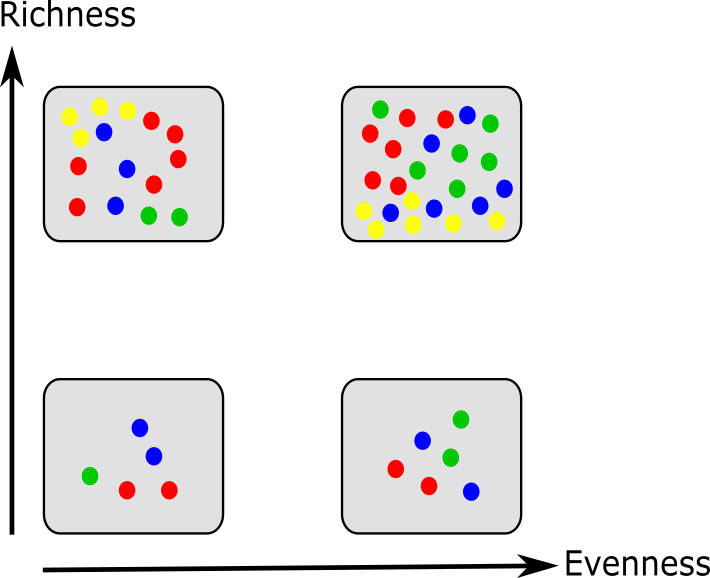
Open image in new tab
