RAD-Seq to construct genetic maps
| Author(s) |
|
| Reviewers |
|
OverviewQuestions:
Objectives:
How to analyze RAD sequencing data for a genetic map study?
Requirements:
SNP calling from RAD sequencing data
Find and correct haplotypes
Create input files for genetic map building software
Time estimation: 8 hoursSupporting Materials:Published: Feb 14, 2017Last modification: May 7, 2026License: Tutorial Content is licensed under Creative Commons Attribution 4.0 International License. The GTN Framework is licensed under MITpurl PURL: https://gxy.io/GTN:T00130rating Rating: 5.0 (0 recent ratings, 1 all time)version Revision: 14
This tutorial is based on the analysis described in publication. Further information about the pipeline is available from the official STACKS website. The authors developed a genetic map in the spotted gar and presented data from a single linkage group. The gar genetic map is an F1 pseudotest cross between two parents and 94 of their F1 progeny. They took the markers that appeared in one of the linkage groups and worked backwards to provide the raw reads from all of the stacks contributing to that linkage group.
This tutorial re-analyzes these data through to genotype determination. These data do not require demultiplexing and do not need processing though Process Radtags tool.
AgendaIn this tutorial, we will deal with:
Pretreatments
Data upload
The original data is available at STACKS website and the subset used here is findable on Zenodo.
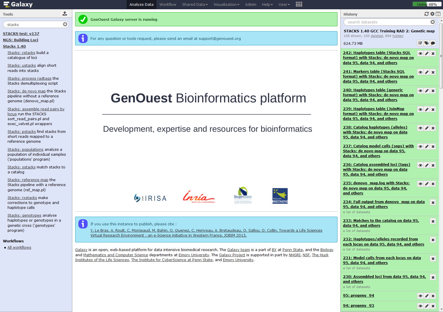
Hands On: Data upload
Create a new history for this RAD-seq exercise.
To create a new history simply click the new-history icon at the top of the history panel:
- Click on galaxy-pencil (Edit) next to the history name (which by default is “Unnamed history”)
- Type the new name
- Click on Save
- To cancel renaming, click the galaxy-undo “Cancel” button
If you do not have the galaxy-pencil (Edit) next to the history name (which can be the case if you are using an older version of Galaxy) do the following:
- Click on Unnamed history (or the current name of the history) (Click to rename history) at the top of your history panel
- Type the new name
- Press Enter
Import Fasta files from parents and 20 progeny.
CommentIf you are using the GenOuest Galaxy instance, you can load the dataset using ‘Shared Data’ -> ‘Data Libraries’ -> ‘1 Galaxy teaching folder’ -> ‘EnginesOn’ -> ‘RADseq’ -> ‘Genetic map’
All of the data for this tutorial is on Zenodo:
https://zenodo.org/record/1219888/files/female
https://zenodo.org/record/1219888/files/male
https://zenodo.org/record/1219888/files/progeny_1
https://zenodo.org/record/1219888/files/progeny_2
https://zenodo.org/record/1219888/files/progeny_3
https://zenodo.org/record/1219888/files/progeny_4
https://zenodo.org/record/1219888/files/progeny_5
https://zenodo.org/record/1219888/files/progeny_6
https://zenodo.org/record/1219888/files/progeny_7
https://zenodo.org/record/1219888/files/progeny_8
https://zenodo.org/record/1219888/files/progeny_9
https://zenodo.org/record/1219888/files/progeny_10
https://zenodo.org/record/1219888/files/progeny_11
https://zenodo.org/record/1219888/files/progeny_12
https://zenodo.org/record/1219888/files/progeny_13
https://zenodo.org/record/1219888/files/progeny_14
https://zenodo.org/record/1219888/files/progeny_15
https://zenodo.org/record/1219888/files/progeny_16
https://zenodo.org/record/1219888/files/progeny_17
https://zenodo.org/record/1219888/files/progeny_18
https://zenodo.org/record/1219888/files/progeny_19
https://zenodo.org/record/1219888/files/progeny_20
- Copy the link location
Click galaxy-upload Upload at the top of the activity panel
- Select galaxy-wf-edit Paste/Fetch Data
Paste the link(s) into the text field
Press Start
- Close the window
As default, Galaxy takes the link as name. It does not link the dataset to a database or a reference genome.


Building loci using STACKS
Run Stacks: De novo map Galaxy tool. This program will run ustacks, cstacks, and sstacks on each individual, accounting for the alignments of each read.
CommentInformation on
denovo_map.pland its parameters can be found online: https://creskolab.uoregon.edu/stacks/comp/denovo_map.php.
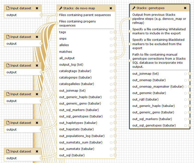
Hands On: Stacks: De novo mapStacks: De novo map tool: Run Stacks selecting the Genetic map usage.
- “Select your usage”:
Genetic map- “Files containing parent sequences”:
femaleandmale- “Files containing progeny sequences”: all 20 progeny files
- “Cross type”:
CP(F1 cross)- Click on
Assembly options
- “Minimum number of identical raw reads required to create a stack”:
3- “Minimum number of identical, raw reads required to create a stack in ‘progeny’ individuals”:
3- “Number of mismatches allowed between loci when building the catalog”:
3- “Remove, or break up, highly repetitive RAD-Tags in the ustacks program”:
YesOnce Stacks has completed running, you will see 5 new data collections and 8 datasets.
Investigate the output files:
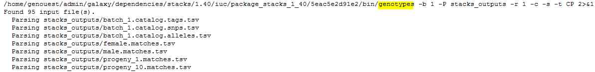
result.logandcatalog.*(snps, alleles and tags).Looking at the first file,
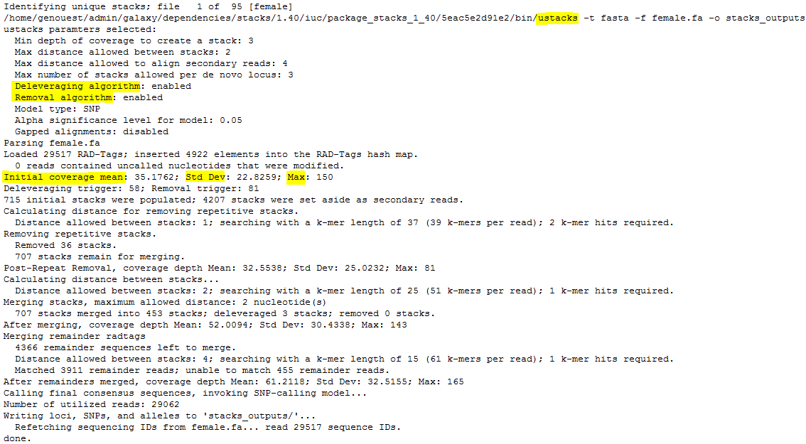
denovo_map.log, you can see the command line used and the start as end execution time.
Then are the different STACKS steps:
ustacks
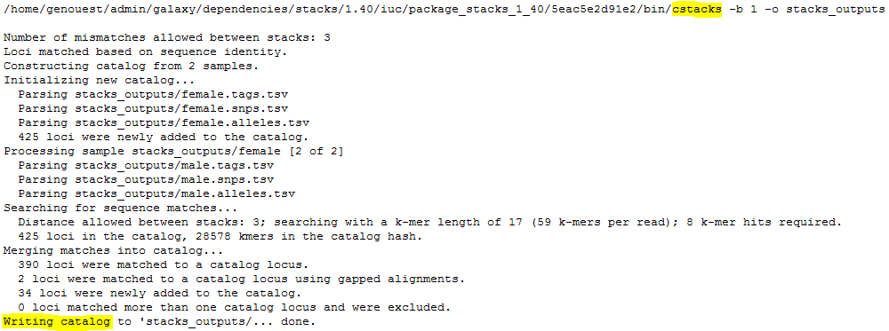
cstacks
Question
- Can you identify the meanning of the number 425?
- Looking at the catalog.tags file, identify specific and shared loci from each individual. Count the number of catalog loci coming from the first individual, from the second, and find on both parents.
- Here, the catalog is made with 459 tags, 425 coming from the “reference individual”, a female. Some of these 425 can be shared with the other parent.
- 35 / 34 / 390
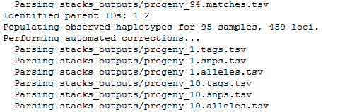
sstacks
Lastly,
genotypesis executed. It searches for markers identified on the parents and the associate progenies’ haplotypes. If the first parent have a GA (ex: aatggtgtGgtccctcgtAc) and AC (ex: aatggtgtAgtccctcgtCc) haplotypes, and the second parent only a GA (ex: aatggtgtGgtccctcgtAc) haplotype, STACKS declares an ab/aa marker for this locus. Genotypes program then associate GA to a and AC to b and then scan progeny to determine which haplotype is found on each of them.
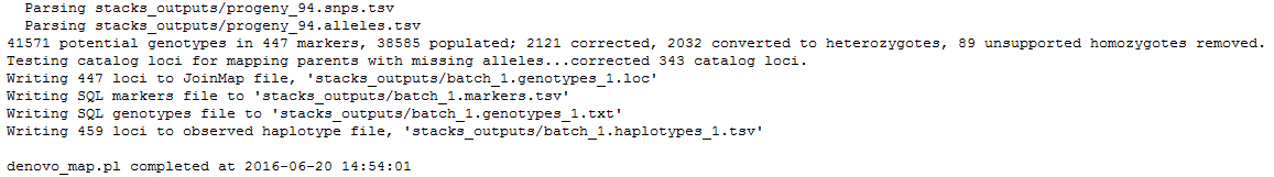
Finally, 447 loci, markers, are kept to generate the
batch_1.genotypess_1.tsvfile. 459 loci are stored on the observed haplotype filebatch_1.haplotypes_1.tsv.
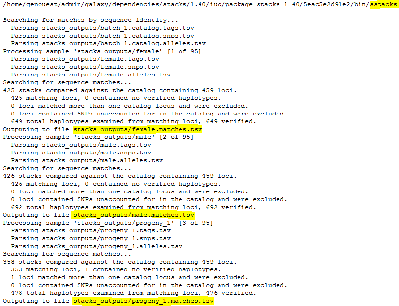
Matches files
Here are sample1.snps (left) and sample2.snps (right)
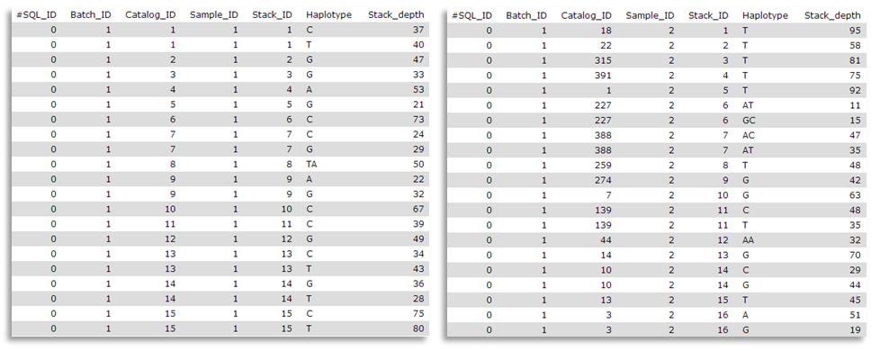
Catalog_ID (= catalog Stacks_ID) is composed by the Stack_ID from the “reference” individual, here sample1, but number is different from sample2 Stack_ID. Thus, in the catalog.alleles.tsv, the Stack_ID number 3 corresponds to the Stack_ID number 16 from sample2!
You can inspect the matches files (you maybe have to change the tsv datatype to a tabular one to correctly display the datasets).
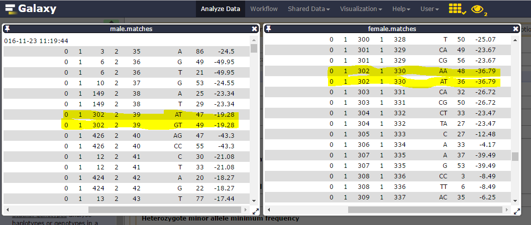
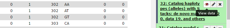
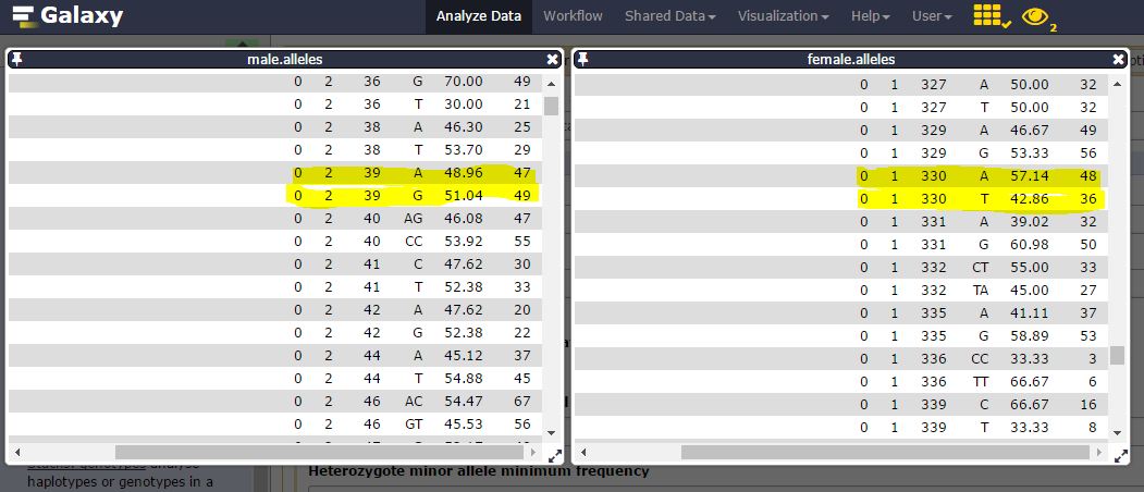
Consider catalog SNPs 27 & 28, on the 302 catalog locus:
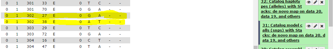
nd the corresponding catalog haplotypes, 3 on the 4 possible (AA, AT, GT but no GA):
heterozygosity is observed on each parent (one ab, the other ac) and there are 19 genotypes for the 22 individuals.
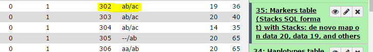
We can then see that Stack_ID 330 for female corresponds to the 39 for male:
Genotypes determination
Hands On: Stacks: GenotypesStacks: genotypes tool: Re-Run the last step of
Stacks: De novo mappipeline specifying more options as:
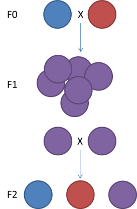
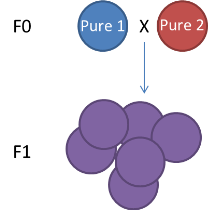
The genetic map type (ie F1, F2 (left figure, F1xF1), Double Haploid, Back Cross (F1xF0), Cross Pollination (right figure, F1 or F2 but resulting from the cross of pure homozygous parents))
Genotyping options output file type for input in genetic mapper tools (ie JoinMap, R/qtl, …). Observe that the R/qtl format for an F2 cross type can be an input for MapMaker or Carthagene.
Thresholds concerning a minimal number of progeny and/or minimum stacks depth to consider a locus
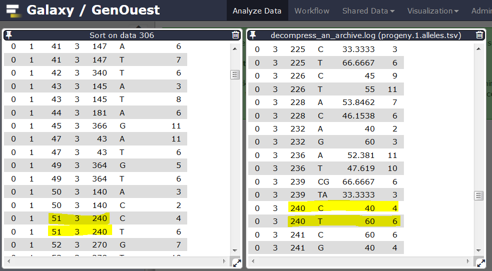
Make Automated Corrections to the Data. This option allows the user to have the program automatically correct some types of errors. This setting can correct errors with the homozygous tags verification in the progeny by confirming the presence or absence of the SNP. If SNP detection model can’t identify a site as heterygous or homozygous, that site is temporarily tagged as homozygous to facilitate the search, by sstacks, in concordance with the loci catalog. If a second allele is detected on the catalog (ie, in parents) and is found on a progeny with a weak frequency (<10% of a stack reads number), the genotypes program can correct the genotype. Additionally, it will delete a homozygous genotype on a particular individual if locus genotype is supported by less than 5 reads. Corrected genotypes are marked uppercase.
Here is an example of a locus originally marked as homozygous before automatic correction because an allele is supported by less than 5 reads. After correction, this locus is marked as heterozygous.
You can re-run Stacks: genotypes tool: modifying the number of genotyped progeny to consider a marker and thus be more or less stringent. Compare results.
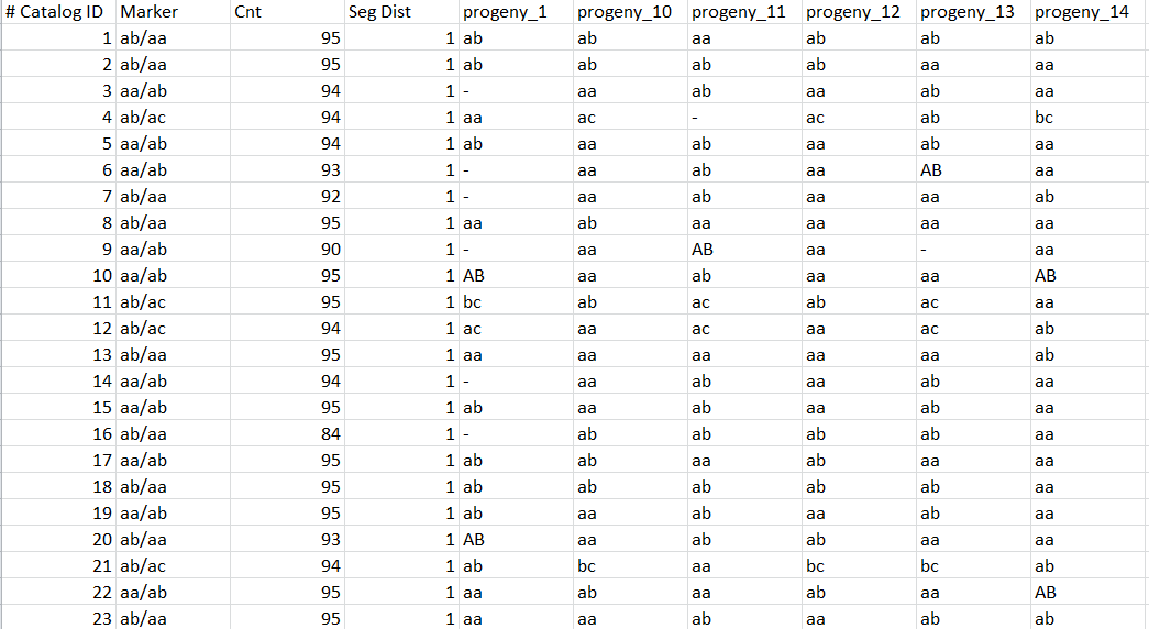
Genotypes.tsv files
One line by locus, one column by individual (aa, ab, AB if automatic correction applied, bb, bc, …) with observed genotype for each locus:
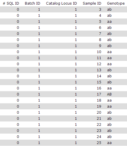
Genotypes.txt files
One line by individual, and for each individual, for each catalog locus, genotype:
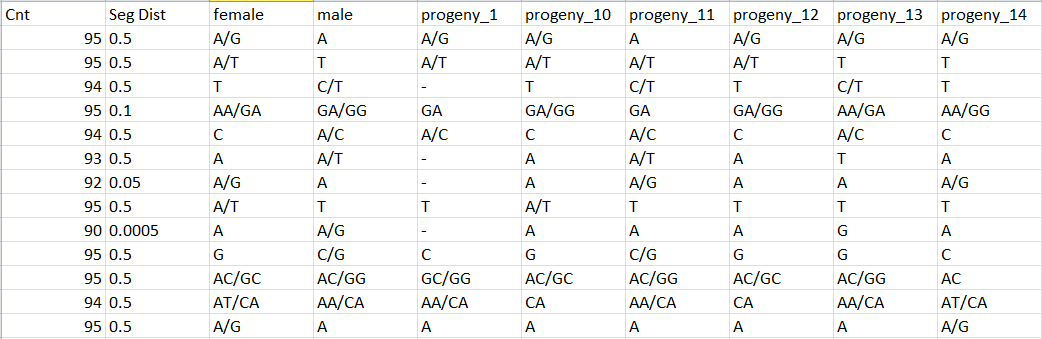
Haplotypes.tsv files
One line by locus, one column by individual (aa, ab, AB if automatic correction applied, bb, bc, …) with observed genotype for each locus:
Question
- The use of the deleverage algorithm allows to not consider loci obtained from merging more than 3 stacks. Why 3 if biologically, you are waiting something related to 2 for diploid organisms?
- Re-execute Stacks: De novo map pipeline modifying the p-value treshold for the SNP model. What is the difference regarding to unverified haplotypes ?
- This value of 3 is important to use if we don’t want to blacklist loci for whom 99.9% of individuals have one and/or the alt allele and 0.01% have a third one, resulting of a sequencing error.
- We see a moficiation of the number of unverified haplotypes
Conclusion
In this tutorial, we have analyzed real RAD sequencing data to extract useful information, such as genotypes and haplotypes to generate input files for downstream genetic map creation. This approach can be summarized with the following scheme:
You've Finished the Tutorial
Frequently Asked Questions
Have questions about this tutorial? Have a look at the available FAQ pages and support channelsUseful literature
Further information, including links to documentation and original publications, regarding the tools, analysis techniques and the interpretation of results described in this tutorial can be found here.
Feedback
Did you use this material as an instructor? Feel free to give us feedback on how it went.
Did you use this material as a learner or student? Click the form below to leave feedback.

Citing this Tutorial
- Yvan Le Bras, RAD-Seq to construct genetic maps (Galaxy Training Materials). https://training.galaxyproject.org/training-material/topics/ecology/tutorials/genetic-map-rad-seq/tutorial.html Online; accessed TODAY
- Hiltemann, Saskia, Rasche, Helena et al., 2023 Galaxy Training: A Powerful Framework for Teaching! PLOS Computational Biology 10.1371/journal.pcbi.1010752
- Batut et al., 2018 Community-Driven Data Analysis Training for Biology Cell Systems 10.1016/j.cels.2018.05.012
Congratulations on successfully completing this tutorial!@misc{ecology-genetic-map-rad-seq, author = "Yvan Le Bras", title = "RAD-Seq to construct genetic maps (Galaxy Training Materials)", year = "", month = "", day = "", url = "\url{https://training.galaxyproject.org/training-material/topics/ecology/tutorials/genetic-map-rad-seq/tutorial.html}", note = "[Online; accessed TODAY]" } @article{Hiltemann_2023, doi = {10.1371/journal.pcbi.1010752}, url = {https://doi.org/10.1371%2Fjournal.pcbi.1010752}, year = 2023, month = {jan}, publisher = {Public Library of Science ({PLoS})}, volume = {19}, number = {1}, pages = {e1010752}, author = {Saskia Hiltemann and Helena Rasche and Simon Gladman and Hans-Rudolf Hotz and Delphine Larivi{\`{e}}re and Daniel Blankenberg and Pratik D. Jagtap and Thomas Wollmann and Anthony Bretaudeau and Nadia Gou{\'{e}} and Timothy J. Griffin and Coline Royaux and Yvan Le Bras and Subina Mehta and Anna Syme and Frederik Coppens and Bert Droesbeke and Nicola Soranzo and Wendi Bacon and Fotis Psomopoulos and Crist{\'{o}}bal Gallardo-Alba and John Davis and Melanie Christine Föll and Matthias Fahrner and Maria A. Doyle and Beatriz Serrano-Solano and Anne Claire Fouilloux and Peter van Heusden and Wolfgang Maier and Dave Clements and Florian Heyl and Björn Grüning and B{\'{e}}r{\'{e}}nice Batut and}, editor = {Francis Ouellette}, title = {Galaxy Training: A powerful framework for teaching!}, journal = {PLoS Comput Biol} }
You can use Ephemeris's
shed-tools installcommand to install the tools used in this tutorial.shed-tools install [-g GALAXY] [-a API_KEY] -t <(curl https://training.galaxyproject.org/training-material/api/topics/ecology/tutorials/genetic-map-rad-seq/tutorial.json | jq .admin_install_yaml -r)Alternatively you can copy and paste the following YAML
---
install_tool_dependencies: true
install_repository_dependencies: true
install_resolver_dependencies: true
tools:
- name: stacks_denovomap
  owner: iuc
  revisions: fdbcc560c691
  tool_panel_section_label: RAD-seq
  tool_shed_url: https://toolshed.g2.bx.psu.edu/
- name: stacks_genotypes
  owner: iuc
  revisions: 62a4b8e5e139
  tool_panel_section_label: RAD-seq
  tool_shed_url: https://toolshed.g2.bx.psu.edu/