Python - Introductory Graduation

Author(s)	Helena Rasche Donny Vrins Bazante Sanders
Reviewers

Overview
Questions:

What all did I learn up until now?

Objectives:

Recap all previous modules.

Use exercises to ensure that all previous knowledge is sufficiently covered.

Requirements:

tutorial Hands-on: Python - Math

tutorial Hands-on: Python - Functions

tutorial Hands-on: Python - Basic Types & Type Conversion

tutorial Hands-on: Python - Lists & Strings & Dictionaries

tutorial Hands-on: Python - Flow Control

tutorial Hands-on: Python - Loops

tutorial Hands-on: Python - Files & CSV

tutorial Hands-on: Python - Try & Except

Time estimation: 1 hour 30 minutes

Level: Introductory Introductory

Supporting Materials:

Jupyter Notebook

instances Available on these Galaxies

Possibly Working

UseGalaxy.eu

UseGalaxy.org

UseGalaxy.org.au

UseGalaxy.fr

Published: Apr 25, 2022

Last modification: Feb 13, 2023

License: Tutorial Content is licensed under Creative Commons Attribution 4.0 International License. The GTN Framework is licensed under MIT

purl PURL: https://gxy.io/GTN:T00084

version Revision: 4

Best viewed in a Jupyter Notebook

This tutorial is best viewed in a Jupyter notebook! You can load this notebook one of the following ways

Run on the GTN with JupyterLite (in-browser computations)

Click to Launch JupyterLite

Launching the notebook in Jupyter in Galaxy

Instructions to Launch JupyterLab

Open a Terminal in JupyterLab with File -> New -> Terminal

Run wget https://training.galaxyproject.org/training-material/topics/data-science/tutorials/python-basics-recap/data-science-python-basics-recap.ipynb

Select the notebook that appears in the list of files on the left.

Downloading the notebook

Right click one of these links: Jupyter Notebook (With Solutions), Jupyter Notebook (Without Solutions)

Save Link As..

This module provide something like a recap of everything covered by the modular Python Introductory level curriculum. This serves as something of a graduation into the Intermediate tutorials which cover more advanced topics.

Agenda

In this tutorial, we will cover:

Review

Math

Functions

Types

Comparators

Iterables

Flow Control

Loops

Files

Exceptions

Exercises

Series Approximation

Monte Carlo Simulation

Sixpack

Review

This recapitulates the main points from all of the previous modular tutorials

Math

Math in python works a lot like math in real life (from algebra onwards). Variables can be assigned, and worked with in the place of numbers

x = 1
y = 2
z = x * y

We can use familiar math operators:

Operator	Operation
`+`	Addition
`-`	Subtraction
`*`	Multiplication
`/`	Division (`//` for rounded, integer division)

And some familiar operations require the use of the math module:

import math
print(math.pow(2, 8))
print(math.sqrt(9))

Functions

Functions were similarly analogous to algebra and mathematics, we can express f(x) = x * 3 in python as:

def f(x, y=3):
    z = y * 2
    return x * z

There are a few basic parts of a function:

def starts a function definition
it needs a name, here it’s f
between some parentheses are the arguments
- the are arguments, just the variable name (x)
- and keyword arguments, where there is a variable and a value (y=3)
The function body
- With one or more lines
- Usually ending in a return

And we know we can nest functions, using functional composition, just like in math. In math functional composition was written f(g(x)) and in python it’s exactly the same:

print(math.sqrt(math.pow(2, 4)))

Here we’ve nested three different functions (print is a function!). To read this we start in the middle (math.pow) and move outwards (math.sqrt, print).

Types

There are lots of different datatypes in Python! The basic types are bool, int, float, str. Then we have more complex datatypes like list and dict which can contain the basic types (as well as other lists/dicts nested.)

Data type	Examples	When to use it	When not to use it
Boolean (`bool`)	`True`, `False`	If there are only two possible states, true or false	If your data is not binary
Integer (`int`)	1, 0, -1023, 42	Countable, singular items. How many patients are there, how many events did you record, how many variants are there in the sequence	If doubling or halving the value would not make sense: do not use for e.g. patient IDs, or phone numbers. If these are integers you might accidentally do math on the value.
Float (`float`)	123.49, 3.14159, -3.33334	If you need more precision or partial values. Recording distance between places, height, mass, etc.
Strings (`str`)	‘patient_12312’, ‘Jane Doe’, ‘火锅’	To store free text, identifiers, sequence IDs, etc.	If it’s truly a numeric value you can do calculations with, like adding or subtracting or doing statistics.
List / Array (`list`)	`['A', 1, 3.4, ['Nested']]`	If you need to store a list of items, like sequences from a file. Especially if you’re reading in a table of data from a file.	If you want to retrieve individual values, and there are clear identifiers it might be better as a dict.
Dictionary / Associative Array / map (`dict`)	`{"weight": 3.4, "age": 12, "name": "Fluffy"}`	When you have identifiers for your data, and want to look them up by that value. E.g. looking up sequences by an identifier, or data about students based on their name. Counting values.	If you just have a list of items without identifiers, it makes more sense to just use a list.

There are a couple more datatypes we didn’t cover in detail: sets, tuple, None, enum, byte, all of which can be read about in Python’s documentation.

Comparators

We have a couple of comparators available to use specifically for numeric values:

>: greater than
<: less than
>=: greater than or equal to
<=: less than or equal to

And a couple that can be used with numbers and strings (or other values!)

==: equal to
!=: does not equal

Iterables

In Python, there is a class of things which can be easily looped over, called “iterables”. All of the following are examples of iterable items:

range(10)
'abcd', a string
['a', 'b' , 'c' , 'd'], a list

Flow Control

Basic flow control looks like if, elif, else:

blood_oxygen_saturation = 92.3
altitude = 0

if blood_oxygen_saturation > 96 and altitude == 0:
    print("Healthy individual at sea level")
elif blood_oxygen_saturation > 92 and altitude >= 1000:
    print("Healthy value above sea level")
elif blood_oxygen_saturation == 0:
    print("Monitor failure")
else:
    print("Not good")

We must start with an if, then we can have one or more elifs, and 0 or 1 else to end our clause. If there is no else, it’s like nothing happens, we just check the if and elifs and if none match, nothing happens by default.

We could use and to check if both conditions are true, and or to check if one condition is true.

# And
for i in (True, False):
    for j in (True, False):
        print(f"{i} AND {j} => {i and j}")
# Or
for i in (True, False):
    for j in (True, False):
        print(f"{i} OR {j} => {i or j}")

And if we needed, we can invert conditions with not.

# Not
for i in (True, False):
    print(f"NOT {i} => {not i}")

All of these components (if/elif/else, and, or, not, numerical and value comparators) let us build up

Loops

Loops let us loop over the contents of something iterable (a string, a list, lines in a file). We write

for loopVariable in myIterable:
    # Do something
    print(loopVariable)

Each loop has:

for, a keyword to start the loop
a loop variable, here named loopVariable which is set automatically every iteration of the loop
in, a keyword used in a loop
something we want to iterate over like a list or string (which is really just a list of single characters) or lines in a file.
a loop body where all the action happens

a = 0
c = 0
t = 0
g = 0

for base in 'ACTGATGCYGGCA':
    if base == 'A':
        a = a + 1
    elif base == 'C':
        c = c + 1
    elif base == 'T':
        t = t + 1
    elif base == 'G':
        g = g + 1
    else:
        print("Unexpected base!")

print(f"a={a} c={c} t={t} g={g}")

Files

In python you must open() a file handle, using one of the three modes (read, write, or append). Normally you must also later close() that file, but your life can be a bit

with open('out.txt', 'w') as handle:
    handle.write("Здравствуйте ")
    handle.write("世界!\n")
    handle.write("Welcome!\n")

# Can no longer handle.write(), once we've exited the with block, the file is automatically closed for us.

There are several basic parts

We use with to indicate we want to use the context manager for file opening (this is what automatically closes the file afterwards)
open(path, mode) opens a file
as is a keyword
handle is the name of a file handle, something that represents the file which we can write to, or read from.

Additionally if you need a newline in your file, you must write it yourself with a \n.

The above code is equivalent to this, but it is not recommended, it’s a bit harder to read, and it is very very common to forget to close files which is not ideal.

handle = open('out.txt', 'w')
handle.write("Здравствуйте ")
handle.write("世界!\n")
handle.write("Welcome!\n")
handle.close()

# Can no longer write.

You can also read from a file:

# Read the entire file as one giant string
with open('out.txt', 'r') as handle:
    print(handle.read())

# Or read it as separate lines.
with open('out.txt', 'r') as handle:
    print(handle.readlines())

Exceptions

Sometimes things go wrong!

You divide by zero (ZeroDivisionError)
You try and add a string and a number (TypeError)
You have incorrect indentation (IndentationError)
Files are unreadable
Files have the wrong permissions

If you expect that something will go wrong you can guard against it with a try/except

try:
    print(1 / 0)
except ZeroDivisionError:
    print("Nope! I expected that!")

Some of the most common reasons to do this are when you’re processing user input data. Users often input invalid data, unfortunately.

Exercises

Series Approximation

Write a program that computes the sum of an alternating series where each element of the series is an expression of the form

\[4\cdot\sum\_{k=1}^{N} \dfrac{(-1)^{k+1}}{2 * k-1}\]

Use that expression and calculate the sum for various values of N like 10, 1000, 1000000

# Write your approximation here!
def calculate_sum(N):
    # for values in the range [1, N] (inclusive!)
        # calculate the expression (the bit after the Sigma)
    # sum up all of those numbers!
    return value

print(calculate_sum(10))

Monte Carlo Simulation

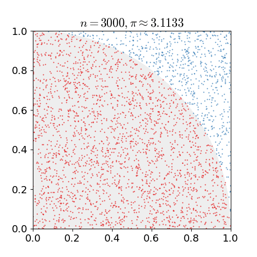
You can use a monte carlo simulation to calculate the value of π. The easy way to do this is to take the region x = [0, 1], y = [0, 1], and fill it with random points. For each point, calculate the distance to the origin. Calculate the ratio of the inside points to the total points, and multiply the value by 4 to estimate π.

You can use the random module to generate random values:

import random

print(random.random())
print(random.random())
print(random.random())

Using the random.random() to generate x and y coordinates, write a function that:

generates N random points
calculate their distance to the origin
Calculate the number of points that are distance<=1
divide that by N, and multiply by 4.

Gif of the unit square 0, 1 on the x and y axes. Points are being randomly generated and points inside the unit circle are marked in red, outside in blue. A quarter of a circle starts to appear, and the numbers at the top show as N increases, the approximation of Pi improves. — **Figure 1**: Gif from the Wikipedia Article for Monte Carlo Method

# Write your code here!
import math

# Just a suggestion: write a function to calculate the distance to origin.
#
def distance(x, y):
    # ...
    return

def generate_random_point():
    # ....
    return [x, y]

def approximate(N=1000):
    # For every point in the range [0, N]
    #   check if it's distance is great than 1

    # Find the ratio of how many are distance<=1
    # and return 4 times that ratio.
    return 4 * x

# Try it with a couple N values like 1, 100, 100000,
n = 10000
# Since we're using a random number function, the result is different every
# time we run the simulation.
print(approximate(n))
print(approximate(n))
print(approximate(n))

Sixpack

Sixpack is an old EMBOSS program which takes in a DNA sequence, and then for every frame, for both strands, emits every Open Reading Frame (ORF) that it sees.

  G  R  G  F  W  C  L  G  G  K  A  A  K  N  Y  R  E  K  S  V  D  V  A  G  Y  D  X   F1
   G  V  A  S  G  A  W  A  V  K  R  Q  K  T  T  V  K  S  R  W  M  W  R  V  M  M     F2
    A  W  L  L  V  P  G  R  *  S  G  K  K  L  P  *  K  V  G  G  C  G  G  L  *  X    F3
1 GGGCGTGGCTTCTGGTGCCTGGGCGGTAAAGCGGCAAAAAACTACCGTGAAAAGTCGGTGGATGTGGCGGGTTATGATG 79
  ----:----|----:----|----:----|----:----|----:----|----:----|----:----|----:----
1 CCCGCACCGAAGACCACGGACCCGCCATTTCGCCGTTTTTTGATGGCACTTTTCAGCCACCTACACCGCCCAATACTAC 79
   P  R  P  K  Q  H  R  P  P  L  A  A  F  F  *  R  S  F  D  T  S  T  A  P  *  S     F6
  X  A  H  S  R  T  G  P  R  Y  L  P  L  F  S  G  H  F  T  P  P  H  P  P  N  H  H   F5
    P  T  A  E  P  A  Q  A  T  F  R  C  F  V  V  T  F  L  R  H  I  H  R  T  I  I    F4

Here we see a DNA sequence GGGCGTGGCTTCTGGTGCCTGGGCGGTAAAGCGGCAAAAAACTACCGTGAAAAGTCGGTGGATGTGGCGGGTTATGATG which you’ll use as input. Above is the translation of the sequence to protein, for each of the three frames (F1-6). Below is the reverse complement of the sequence, and the three frame translation again.

What sixpack does is:

orfs = []

for sequence in [forward, reverse_complement(forward)]:
    for frame in [sequence, sequence[1:], sequence[2:]]:
        # Remembering
        for potential start_codon:
            # accumulate until it sees a stop codon
            # and append it to the orfs array once it does.

Here are some variables for your convenience:

start_codons = ['TTG', 'CTG', 'ATG']
stop_codons = ['TAA', 'TAG', 'TGA']

# And some convenience functions
def is_start_codon(codon):
    return codon in start_codons

def is_stop_codon(codon):
    return codon in stop_codons

It’s a good exercise to rewrite sixpack in a very simplified version without most of the features in sixpack:

# Write your code here!

# Some recommendations:
def reverse_complement(sequence):
    return ...

orfs = []

for sequence in [forward, reverse_complement(forward)]:
    for frame in [sequence, sequence[1:], sequence[2:]]:
        # Remembering
        for potential start_codon:
            # accumulate until it sees a stop codon
            # and append it to the orfs array once it does.

You've Finished the Tutorial

Key points

Frequently Asked Questions

Have questions about this tutorial? Check out the FAQ page for the Foundations of Data Science topic to see if your question is listed there. If not, please ask your question on the GTN Gitter Channel or the Galaxy Help Forum

Glossary

ORF: Open Reading Frame

Feedback

Did you use this material as an instructor? Feel free to give us feedback on how it went.
Did you use this material as a learner or student? Click the form below to leave feedback.

Citing this Tutorial

Helena Rasche, Donny Vrins, Bazante Sanders, Python - Introductory Graduation (Galaxy Training Materials). https://training.galaxyproject.org/training-material/topics/data-science/tutorials/python-basics-recap/tutorial.html Online; accessed TODAY
Hiltemann, Saskia, Rasche, Helena et al., 2023 Galaxy Training: A Powerful Framework for Teaching! PLOS Computational Biology 10.1371/journal.pcbi.1010752
Batut et al., 2018 Community-Driven Data Analysis Training for Biology Cell Systems 10.1016/j.cels.2018.05.012

@misc{data-science-python-basics-recap,
author = "Helena Rasche and Donny Vrins and Bazante Sanders",
	title = "Python - Introductory Graduation (Galaxy Training Materials)",
	year = "",
	month = "",
	day = "",
	url = "\url{https://training.galaxyproject.org/training-material/topics/data-science/tutorials/python-basics-recap/tutorial.html}",
	note = "[Online; accessed TODAY]"
}
@article{Hiltemann_2023,
	doi = {10.1371/journal.pcbi.1010752},
	url = {https://doi.org/10.1371%2Fjournal.pcbi.1010752},
	year = 2023,
	month = {jan},
	publisher = {Public Library of Science ({PLoS})},
	volume = {19},
	number = {1},
	pages = {e1010752},
	author = {Saskia Hiltemann and Helena Rasche and Simon Gladman and Hans-Rudolf Hotz and Delphine Larivi{\`{e}}re and Daniel Blankenberg and Pratik D. Jagtap and Thomas Wollmann and Anthony Bretaudeau and Nadia Gou{\'{e}} and Timothy J. Griffin and Coline Royaux and Yvan Le Bras and Subina Mehta and Anna Syme and Frederik Coppens and Bert Droesbeke and Nicola Soranzo and Wendi Bacon and Fotis Psomopoulos and Crist{\'{o}}bal Gallardo-Alba and John Davis and Melanie Christine Föll and Matthias Fahrner and Maria A. Doyle and Beatriz Serrano-Solano and Anne Claire Fouilloux and Peter van Heusden and Wolfgang Maier and Dave Clements and Florian Heyl and Björn Grüning and B{\'{e}}r{\'{e}}nice Batut and},
	editor = {Francis Ouellette},
	title = {Galaxy Training: A powerful framework for teaching!},
	journal = {PLoS Comput Biol}
}

                   

Congratulations on successfully completing this tutorial!

Go Further
Do you want to extend your knowledge? Follow one of our recommended follow-up trainings:

You can use Ephemeris's shed-tools install command to install the tools used in this tutorial.
shed-tools install [-g GALAXY] [-a API_KEY] -t <(curl https://training.galaxyproject.org/training-material/api/topics/data-science/tutorials/python-basics-recap/tutorial.json | jq .admin_install_yaml -r)
Alternatively you can copy and paste the following YAML
---
install_tool_dependencies: true
install_repository_dependencies: true
install_resolver_dependencies: true
tools: []

No feedback has been recieved yet for this training. Be the first one by filling in the feedback form from above.