Mapping and molecular identification of phenotype-causing mutations
| Author(s) |
|
| Reviewers |
|
OverviewQuestions:
Objectives:
What is mapping-by-sequencing?
How can it help you identify the causative mutation in phenotypic mutants isolated from genetic screens?
Requirements:
Use joint variant calling and extraction to facilitate variant comparison across samples
Perform variant linkage analyses for phenotypically selected recombinant progeny
Filter, annotate and report lists of variants
- Introduction to Galaxy Analyses
- slides Slides: Quality Control
- tutorial Hands-on: Quality Control
- slides Slides: Mapping
- tutorial Hands-on: Mapping
Time estimation: 2 hoursSupporting Materials:Published: Mar 7, 2018Last modification: Nov 9, 2023License: Tutorial Content is licensed under Creative Commons Attribution 4.0 International License. The GTN Framework is licensed under MITpurl PURL: https://gxy.io/GTN:T00312rating Rating: 4.8 (0 recent ratings, 4 all time)version Revision: 16
In order to map and identify phenotype-causing mutations efficiently from a single experiment, modern genetic research aims to combine classical genetic mapping concepts with the power of next-generation-sequencing.
For example, after having obtained a mutant strain of an organism with a particular phenotype from a forward genetic screen, the classical approach towards identification of the underlying causative mutation would be to:
- perform mapping crosses to probe for linkage between the unknown mutation and selected markers with known location on the genome, in order to determine the approximate genomic region that the mutation resides in, then
- sequence candidate DNA stretches in this region to identify the precise nature of the mutation.
Modern approaches, in contrast, use just one set of genome-wide sequencing data obtained from mapping-cross progeny and suitable parent strains to simultaneously:
- discover available marker mutations for linkage analysis,
- map the causative mutation using these markers, and
- identify candidate mutations.
Since it uses sequencing data already at the mapping step, this process is called mapping-by-sequencing.
Since genome-wide sequencing will often reveal a few hundreds to many thousands of marker variants that should be considered together in the linkage analysis, mapping-by-sequencing data is typically analyzed with dedicated computational tools. For Galaxy, the MiModD suite of tools offers efficient and flexible analysis workflows compatible with a variety of mapping-by-sequencing approaches.
The MiModD documentation has its own chapter on supported mapping-by-sequencing schemes not covered here.
In this tutorial we are going to use several of these tools to map and identify a point mutation in an Arabidopsis thaliana strain from whole-genome sequencing data. This will demonstrate one particular kind of linkage analysis supported by MiModD called Variant Allele Frequency Mapping.
Variant Allele Frequency
Mapping
 Open image in new tab
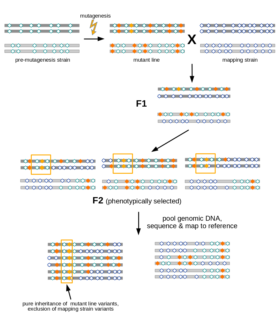
As illustrated in Figure 1, variant allele frequency mapping analyzes marker variant inheritance patterns in pooled F2 recombinants selected for the mutation to be mapped.
In the figure we assume a diploid organism with just two pairs (dark and light grey) of chromosomes.
A mutant line established for any organism will harbor two types of variants (diamonds):
- variants induced during mutagenesis (orange), among them the causative variant responsible for the mutant phenotype (yellow)
- variants (with respect to the species’ reference genome) that were present in the premutagenesis strain (green open diamonds)
For mapping the causative mutation, additional variants (blue open diamonds) are introduced through a cross to a mapping strain and F2 progeny is selected for the mutant phenotype. While each individual in the F2 generation carries its uniquely recombined variant pattern (3 possible outcomes for the diploid genome are shown in the figure), this phenotypic selection will work against mapping strain variants in the vicinity (yellow boxes) of the causative variant. Hence, when the recombined DNA from phenotypic F2 progeny gets pooled and sequenced, the causative variant can be found by looking for a region for which all sequenced reads support variant alleles found in the original mutant line, rather than mapping strain variant alleles.
Agenda
Data Preparation
In this tutorial we are going to (re-)identify the recessive causative mutation in a late-flowering mutant line of Arabidopsis thaliana.
CommentMiModD was developed as a successor of the older and now unmaintained CloudMap suite of tools, but also uses some key concepts first implemented in the command line package SHOREmap. The data used in this tutorial represent a subsample of the SHOREmap proof-of-principle data (specifically of the
OCF2andLerdatasets).
The mutant line was obtained from a mutagenesis screen on the Columbia reference background of A. thaliana. For mapping-by-sequencing, the line was outcrossed to the highly polymorphic Landsberg erecta background as a source of marker variants. From this outcross, 119 F2 siblings showing the original late-flowering phenotype were recovered and their genomic DNA was pooled and subjected to whole-genome sequencing. Together with whole-genome sequencing data of a pure Ler background strain, this outcrossed pool data forms the starting point of our analysis. The Ler strain sample, thus, can inform us about the markers that the outcrossed F2 pool could have inherited and exclusion of Ler markers from a particular genomic region from the F2 pool provides evidence that the phenotype causing variant lies close to this region. With respect to Figure 1, this means that we will only use “blue diamond” marker variants introduced through the mapping cross for the linkage analysis and ignore potentially informative (green and orange) variants found in the original mutant line.
For your convenience, the sequenced reads from both datasets have already been mapped (using Bowtie2) to the A. thaliana Col reference genome (version TAIR10) so the two datasets take the form of BAM files with the mapping results (see the tutorial on NGS data mapping if you do not know what this means).
Hands On: Data upload and preprocessingThis section assumes that you already know
- how to upload data to Galaxy via links
- edit dataset attributes
- do some basic text manipulation on datasets
An excellent introduction into these topics can be found in the From peaks to genes tutorial (specifically, in the sections on Data upload and File preparation).
- Import the two BAM datasets representing the:
- Specify the genome that was used at the reads mapping step
- Click on Edit attributes (the pencil icon displayed with the dataset)
- As the Database/Build select
Arabidopsis thaliana TAIR10- Save the edited attributes
Import the reference genome
Comment: TAIR10 VersionThis step is only necessary if the TAIR10 version of the A. thaliana genome is not available as a built-in genome on your Galaxy server.
- Upload the reference genome using the URL:
https://www.arabidopsis.org/download_files/Genes/TAIR10_genome_release/TAIR10_chromosome_files/TAIR10_chr_all.fas- Use Replace parts of text tool to truncate the title lines in the fasta dataset to just the bare chromosome names. Set:
the Find pattern to
^>(\w+).*This will find entire fasta title lines, or more specifically, any lines starting with
>followed by at least one letter, digit or underscore.the Replace with pattern to
>chr$1The
$1in it refers to the parenthesized part of the find pattern, i.e., just the substring of letters/digits/underscores directly following the>.Find-Pattern is a regular expression to
Yes- Make sure the datatype of the resulting dataset is set to
fastaand give the dataset a nice name (e.g., TAIR10 reference).- At this point you can delete the originally downloaded dataset.
Joint Variant Calling and Extraction
A hallmark of all mapping-by-sequencing analyses is that one would like to follow the fate of variants through genetic crosses. In this tutorial, for example, we would like to determine, for every marker variant provided by the Ler background, at what frequency it got inherited by the outcrossed F2 pool. For such analyses to work reliably, it is best to call variants jointly for all relevant samples because this allows the variant caller to give us per-sample variant call statistics for all sites at which any sample is found to have a non-wt genotype. In our case, this means that the variant caller will report any variants it finds for the Ler background sample along with the call statistics for the outcrossed F2 pool at that same site - even if the variant allele contributes very little to the pool and would, thus, have been disregarded in a standard single-sample analysis.
Here, we are using the MiModD Variant Calling tool for joint variant calling for our two samples. This tool outputs variant call statistics across all sites and all samples in the compact binary BCF format. We can then use the MiModD Extract Variant Sites tool to extract sites, for which at least one sample appears to have a non-wt genotype, and report them in VCF format.
Hands On: Variant Calling
- Use MiModD Variant Calling tool to generate combined variant call statistics:
Select the reference genome to call variants against.
If your Galaxy server offers version TAIR10 of the A. thaliana reference as a built-in genome, you can go ahead and use it. Otherwise, download and preprocess the reference as described under Data Preparation and use it as a genome from my history.
- As the Aligned reads input datasets for the analysis select the two BAM datasets representing the two samples (use the
Controlkey on the keyboard to select multiple datasets from the list.- Execute the job
- Run MiModD Extract Variant Sites tool with
- BCF input file set to the BCF dataset generated in the previous step.
Question
- Approximately how many variants were extracted?
- Does this number surprise you?
- You can click on the extracted variants dataset in your history to get more details about it. You should see that the file has an estimated 130,000 lines. Since one variant gets reported per line in VCF format (apart from a number of header lines), this roughly equals the number of variants in the dataset.
The huge number of variants reflects the fact that the Ler mapping strain is really quite diverged from the Col reference background that the mutant was generated in and, thus, offers many marker variants for mapping.
In total, the Ler genome harbors >400,000 single nucleotide variants compared to the Col reference, but to keep the tutorial datasets small we only provided reads mapping to 2 out of 5 chromosomes. In addition, we provided really low-coverage data even for those two chromosomes so our analysis will miss many true variants and contain many questionable variant calls that may represent false-positives. Regardless, an analysis based on such a large overall number of variants is robust enough to provide useful results.
Linkage Analysis
The extracted variants dataset obtained in the previous step contains information about thousands of sites that can be used as markers to map the causative mutation in the F2 pool. We will now analyze the data with the MiModD NacreousMap tool in Variant Allele Frequency mapping mode to identify these markers and look for linkage between them and the causative mutation.
Hands On: Linkage Analysis with one set of parentally contributed markersIn the MiModD NacreousMap tool interface, set
- type of mapping analysis to perform to
Variant Allele Frequency Mappingand- data source to use to
VCF file of variants.- As the input file with variants to analyze select your extracted variants VCF dataset obtained in the previous step.
- As the mapping sample name use
outcrossed F2.- Leave the name of the related parent sample input field empty because in this two-sample there is no such sample.
- As the name of the unrelated parent sample specify
Ler.Comment: Sample rolesIn
Variant Allele Frequency Mappingmode the tool requires:
- a mapping sample, which corresponds to the recombinant pool, from which allele frequencies should be calculated
- either a related or an unrelated parent sample (or both), from which the marker variant sites to use in the linkage analysis will be determined. A related parent sample is related (or identical) to the original mutant line by descent and provides information about (some of) the variants present in that line, while an unrelated parent sample provides information about the mapping strain variants introduced in the mapping cross. If both a related and an unrelated parent sample are available, the tool can also use the marker sets from both sides for the linkage analysis.
With these settings, we base the linkage analysis on crossed-in variants only, i.e., the tool will look for variants, for which the Ler sample appears homozygous mutant, and determine the contribution of each such variant allele to the recombinant pool highlighting regions of low contribution, i.e., with suspected linkage to the causative variant, in its output.
Running this job will generate two datasets, one with linkage tables for each chromosome in the A. thaliana genome, one with graphical representations of the data.
Question
- Have a look at the linkage plots dataset generated by the tool run. In which interval on which chromosome would you expect the causative mutation?
- Are the per-marker scatter plots and the histogram plots in agreement?
- What about those
No markers found!messages (you saw them, right?) that the tool printed?
- The plots suggest that the causative variant is likely to be found in the region from 18,000,000 to 19,000,000 on chr2.
Look at the y axis labels! The scatter plots show the rates at which marker sites appear to recombine with the causative mutation in the pool of F2 recombinants, while the histograms show linkage evidence. Hence, a dip of the scatter plot regression line towards zero corresponds to a peak in the histograms and the two kinds of plots are, thus, in very good agreement for this analysis.
In general, the histogram plots are easier to digest and often provide more precise mapping intervals, and are often all you need for mapping a causative variant. The per-marker scatter plots, on the other hand, are closer to the raw data and can sometimes reveal additional irregularities in the data that may indicate problems with the mapping cross or unexpected factors influencing the inheritance pattern.
- Since we included only reads mapping to chromosome 1 or 2 in the original BAM files, the tool will not be able to detect any markers for the other chromosomes.
Identifying Candidate Mutations
With the mapping results obtained above we can now try to get a list of candidates for the causative mutation. Here is what we know about this mutation so far:
-
The F2 recombinant pool should appear homozygous mutant for it.
This is because the F2 recombinants got selected based on the phenotype of the recessive mutation so we can assume that all individuals in the pool were homozygous for it.
-
The Ler strain should not carry it.
-
It should reside in the genomic region identified in the previous step.
Hands On: Variant FilteringWith the above information, we can run MiModD VCF Filter tool to obtain a new VCF dataset with only those variants from the originally extracted ones that fulfill all three criteria. In the tool interface,
- select as VCF input file the extracted variants dataset from your history
- add a Sample-specific Filter and set its
- sample to
outcrossed F2- genotype pattern(s) for the inclusion of variants to
1/1These settings will make the filter retain only variants for which the F2 pool has a
1/1, i.e., homozygous mutant genotype.- add another Sample-specific Filter and set its
- sample to
Ler- genotype pattern(s) for the inclusion of variants to
0/0This filter will retain only variants for which the mapping strain sample has a homozygous wt genotype.
- add a Region Filter and set its
- Chromosome to
chr2- Region Start to 18000000
- Region End to 19000000
to retain only variants falling into the previously determined mapping interval.
Comment: Sample and chromosome namesThis is the second time in this tutorial that we ask you to type sample or chromosome names exactly as they appear in a dataset, and so you may have started wondering how you are supposed to keep track of which names are used where in your own analyses.
Because this is a valid concern, the MiModD tool suite features the MiModD File Information tool tool that can report the sample and sequence names stored in almost any dataset that you may encounter in a mapping-by-sequencing analysis (specifically, the tool can handle datasets in vcf, bcf, sam, bam and fasta format).
Running the job yields a new VCF dataset with variants that passed all filters.
Question
- How many variants passed the filters?
- How many variants would you have to consider as candidates if you did not have any mapping information?
- If you used the suggested mapping interval of 1Mb on chr2, you should have retained 5 variants. Filtering is a really powerful way to reduce the number of variants to consider!
- Re-running the job with the region filter removed shows that across the two chromosomes, for which the input datasets provided sequencing reads, there are 50 variants for which the pool appears homozygous mutant and for which the Ler strain is homozygous wt.
Not all of the retained variants are equally likely candidates for being the causative mutation. Since the input datasets consist of reads from whole-genome sequencing, as opposed to exome sequencing, some of the variants may fall in intergenic regions or introns where they are unlikely to cause a phenotype. Other variants may fall in coding regions, but may be silent on the protein level. Hence, we can prioritize our candidate variants after annotating them with predicted functional effects.
Hands On: Variant AnnotationTo annotate our variants we are going to use SnpEff with its
Arabidopsis_thalianagenome database as the source of functional genomic annotations, then generate a human-friendly variant report with the MiModD Report Variants tool tool.
Use SnpEff Download tool to download genome database
Arabidopsis_thaliana.Comment: SnpEff versionsSnpEff genome databases can only be used with the specific
major.minorversion of SnpEff they were built for. Make sure you are using matching versions (e.g.,4.3- differences past the second digit are fine and denote subversions with compatible database schemes) of SnpEff Download tool in this and of SnpEff Variant effect and annotation tool in the next step.Please also note that before SnpEff version 4.3 the TAIR10 version of the A. thaliana genome database was named
athalianaTair10. If your Galaxy server offers only older versions of the SnpEff tools, you will have to use that name instead ofArabidopsis_thaliana.- In the SnpEff Variant effect and annotation tool interface, set:
- Sequence changes (SNPs, MNPs, InDels) to your filtered VCF dataset
- Genome source to
Downloaded snpEff database in your history- SnpEff4.3 Genome Data to your just downloaded genome dataset
under Annotation options check
Use 'EFF' field compatible with
older versions (instead of 'ANN')
This last setting is required for compatibility of the resulting dataset with the current version of MiModD Report Variants tool.
Running this job will produce another VCF dataset with the functional annotation data added to its INFO column. Inspecting this dataset is not particularly convenient, but you can turn it into a more user-friendly report by
- using MiModD Report Variants tool and setting:
- The VCF input with the variants to be reported to the annotated variants dataset generated by SnpEff
- the Format to use for the report to
HTMLSpecies to
A. thaliana.The species information can be used by the tool to enrich the output with species-specific database and genome browser links.
CommentVariant reports in html format are meant to be used on relatively small lists of candidate variants like in this example. If the input VCF contains > 1000 variants, the relatively large size of the reports and slow loading in the browser may become annoying. In this case, or if you experience formatting problems with the generated html in your browser, it may be better to choose
Tab-separated plain textas the report format although the output will then lack those convenient hyperlinks.QuestionThe published confirmed mutations in the mutant line are chr2:18,774,111 C→T and chr2:18,808,927 C→T. The latter was shown through follow-up experiments to be the causative variant.
- What are the functional effects of these two mutations according to the report?
- What biological functions are described for the two genes? How do these relate to the phenotype of our mutant line?
- The C→T transition at 18,774,111 results in a premature translational stop for the transcript AT2G45550.1. The C→T transition at 18,808,927 affects a splice donor site and, thus, is likely to interfere with correct splicing of the transcript AT2G45660.1.
- From the linked gene pages at TAIR you can learn that the gene AT2G45550 encodes a cytochrome P450, while AT2G45660 encodes a protein called AGL20/SOC1, which is known to control flowering. Thus, there is a direct connection between the late-flowering phenotype of the mutant line studied here and the known role of the gene affected by chr2:18,808,927 C→T.
Conclusion
Mapping-by-sequencing can greatly speed up and facilitate the molecular identification of mutations recovered from mutagenesis screens. The method makes extensive use of cross-sample comparison of variants and benefits strongly from joint variant calling to generate reliable and manageable variant information. A combination of variant linkage analysis and filtering often results in very small lists of candidate variants that can then be confirmed through further experimental work. Importantly, the selection of biological samples for sequencing determines the meaningful variant comparisons that can be made in the bioinformatics analysis so it is important to understand the essence of the analysis method before the preparation of any biological samples.
You've Finished the Tutorial
Key points
Mapping-by-sequencing is a powerful method for the molecular identification of mutations
The MiModD suite of tools bundles most of the functionality required to perform mapping-by-sequencing analyses with Galaxy
Frequently Asked Questions
Have questions about this tutorial? Have a look at the available FAQ pages and support channelsUseful literature
Further information, including links to documentation and original publications, regarding the tools, analysis techniques and the interpretation of results described in this tutorial can be found here.
Feedback
Did you use this material as an instructor? Feel free to give us feedback on how it went.
Did you use this material as a learner or student? Click the form below to leave feedback.

Citing this Tutorial
- Wolfgang Maier, Mapping and molecular identification of phenotype-causing mutations (Galaxy Training Materials). https://training.galaxyproject.org/training-material/topics/variant-analysis/tutorials/mapping-by-sequencing/tutorial.html Online; accessed TODAY
- Hiltemann, Saskia, Rasche, Helena et al., 2023 Galaxy Training: A Powerful Framework for Teaching! PLOS Computational Biology 10.1371/journal.pcbi.1010752
- Batut et al., 2018 Community-Driven Data Analysis Training for Biology Cell Systems 10.1016/j.cels.2018.05.012
Congratulations on successfully completing this tutorial!@misc{variant-analysis-mapping-by-sequencing, author = "Wolfgang Maier", title = "Mapping and molecular identification of phenotype-causing mutations (Galaxy Training Materials)", year = "", month = "", day = "", url = "\url{https://training.galaxyproject.org/training-material/topics/variant-analysis/tutorials/mapping-by-sequencing/tutorial.html}", note = "[Online; accessed TODAY]" } @article{Hiltemann_2023, doi = {10.1371/journal.pcbi.1010752}, url = {https://doi.org/10.1371%2Fjournal.pcbi.1010752}, year = 2023, month = {jan}, publisher = {Public Library of Science ({PLoS})}, volume = {19}, number = {1}, pages = {e1010752}, author = {Saskia Hiltemann and Helena Rasche and Simon Gladman and Hans-Rudolf Hotz and Delphine Larivi{\`{e}}re and Daniel Blankenberg and Pratik D. Jagtap and Thomas Wollmann and Anthony Bretaudeau and Nadia Gou{\'{e}} and Timothy J. Griffin and Coline Royaux and Yvan Le Bras and Subina Mehta and Anna Syme and Frederik Coppens and Bert Droesbeke and Nicola Soranzo and Wendi Bacon and Fotis Psomopoulos and Crist{\'{o}}bal Gallardo-Alba and John Davis and Melanie Christine Föll and Matthias Fahrner and Maria A. Doyle and Beatriz Serrano-Solano and Anne Claire Fouilloux and Peter van Heusden and Wolfgang Maier and Dave Clements and Florian Heyl and Björn Grüning and B{\'{e}}r{\'{e}}nice Batut and}, editor = {Francis Ouellette}, title = {Galaxy Training: A powerful framework for teaching!}, journal = {PLoS Comput Biol} }
You can use Ephemeris's
shed-tools installcommand to install the tools used in this tutorial.shed-tools install [-g GALAXY] [-a API_KEY] -t <(curl https://training.galaxyproject.org/training-material/api/topics/variant-analysis/tutorials/mapping-by-sequencing/tutorial.json | jq .admin_install_yaml -r)Alternatively you can copy and paste the following YAML
---
install_tool_dependencies: true
install_repository_dependencies: true
install_resolver_dependencies: true
tools:
- name: text_processing
  owner: bgruening
  revisions: a6f147a050a2
  tool_panel_section_label: Text Manipulation
  tool_shed_url: https://toolshed.g2.bx.psu.edu/
- name: snpeff
  owner: iuc
  revisions: 20f0429a4bfe
  tool_panel_section_label: Variant Calling
  tool_shed_url: https://toolshed.g2.bx.psu.edu/
- name: snpeff
  owner: iuc
  revisions: 20f0429a4bfe
  tool_panel_section_label: Variant Calling
  tool_shed_url: https://toolshed.g2.bx.psu.edu/
- name: mimodd_main
  owner: wolma
  revisions: f0f2795de2c7
  tool_panel_section_label: MiModD
  tool_shed_url: https://toolshed.g2.bx.psu.edu/
- name: mimodd_main
  owner: wolma
  revisions: f0f2795de2c7
  tool_panel_section_label: MiModD
  tool_shed_url: https://toolshed.g2.bx.psu.edu/
- name: mimodd_main
  owner: wolma
  revisions: f0f2795de2c7
  tool_panel_section_label: MiModD
  tool_shed_url: https://toolshed.g2.bx.psu.edu/
- name: mimodd_main
  owner: wolma
  revisions: f0f2795de2c7
  tool_panel_section_label: MiModD
  tool_shed_url: https://toolshed.g2.bx.psu.edu/
- name: mimodd_main
  owner: wolma
  revisions: f0f2795de2c7
  tool_panel_section_label: MiModD
  tool_shed_url: https://toolshed.g2.bx.psu.edu/