RNA-seq Alignment with STAR
| Author(s) |
|
| Editor(s) |
|
| Reviewers |
|
OverviewQuestions:
Objectives:
What are the first steps to process RNA-seq data?
Requirements:
Learn the basics to process RNA sequences
Check the quality and trim the sequences with bash
Use command line STAR aligner to map the RNA sequences
Estimate the number of reads per gens
- Introduction to Galaxy Analyses
- slides Slides: Quality Control
- tutorial Hands-on: Quality Control
- slides Slides: Mapping
- tutorial Hands-on: Mapping
Time estimation: 1 hour 30 minutesSupporting Materials:Published: May 15, 2023Last modification: Nov 9, 2023License: Tutorial Content is licensed under Creative Commons Attribution 4.0 International License. The GTN Framework is licensed under MITpurl PURL: https://gxy.io/GTN:T00346rating Rating: 3.3 (0 recent ratings, 3 all time)version Revision: 6
In recent years, RNA sequencing (in short RNA-Seq) has become a very widely used technology to analyze the continuously changing cellular transcriptome, i.e. the set of all RNA molecules in one cell or a population of cells. One of the most common aims of RNA-Seq is the profiling of gene expression by identifying genes or molecular pathways that are differentially expressed (DE) between two or more biological conditions. This tutorial demonstrates a computational workflow for counting and locating the genes in RNA sequences. The first and most critical step in an RNA-seq analysis.
In the study of Brooks et al. 2011, the authors identified genes and pathways regulated by the Pasilla gene (the Drosophila homologue of the mammalian splicing regulators Nova-1 and Nova-2 proteins) using RNA-Seq data. They depleted the Pasilla (PS) gene in Drosophila melanogaster by RNA interference (RNAi). Total RNA was then isolated and used to prepare both single-end and paired-end RNA-Seq libraries for treated (PS depleted) and untreated samples. These libraries were sequenced to obtain RNA-Seq reads for each sample. The RNA-Seq data for the treated and the untreated samples can be compared to identify the effects of Pasilla gene depletion on gene expression.
In this tutorial, we illustrate the analysis of the gene expression data step by step using 7 of the original datasets:
- 4 untreated samples: GSM461176, GSM461177, GSM461178, GSM461182
- 3 treated samples (Pasilla gene depleted by RNAi): GSM461179, GSM461180, GSM461181
Each sample constitutes a separate biological replicate of the corresponding condition (treated or untreated). Moreover, two of the treated and two of the untreated samples are from a paired-end sequencing assay, while the remaining samples are from a single-end sequencing experiment.
Comment: Full dataThe original data are available at NCBI Gene Expression Omnibus (GEO) under accession number GSE18508. The raw RNA-Seq reads have been extracted from the Sequence Read Archive (SRA) files and converted into FASTQ files.
AgendaIn this tutorial, we will cover:
CommentThis tutorial is significantly based on Galaxy’s “Reference-based RNA-Seq data analysis” tutorial.
Data Upload
At first, we need to put our hands on our data. In this tutorial we will use the files for 2 out of the 7 samples to demonstrate how to calculate read counts (a measure of the gene expression) from FASTQ files (quality control, mapping, read counting). The FASTQ files for the other 5 samples, are provided, in case you want to reproduce the whole analysis later. The “Data Upload” process is the only one in this tutorial that takes place directly into Galaxy’s interface.
Hands On: Data upload
- Import the FASTQ file pairs from Zenodo or a data library:
GSM461177(untreated):GSM461177_1andGSM461177_2GSM461180(treated):GSM461180_1andGSM461180_2https://zenodo.org/record/6457007/files/GSM461177_1.fastqsanger https://zenodo.org/record/6457007/files/GSM461177_2.fastqsanger https://zenodo.org/record/6457007/files/GSM461180_1.fastqsanger https://zenodo.org/record/6457007/files/GSM461180_2.fastqsanger
- Copy the link location
Click galaxy-upload Upload at the top of the activity panel
- Select galaxy-wf-edit Paste/Fetch Data
Paste the link(s) into the text field
Press Start
- Close the window
As an alternative to uploading the data from a URL or your computer, the files may also have been made available from a shared data library:
- Go into Libraries (left panel)
- Navigate to the correct folder as indicated by your instructor.
- On most Galaxies tutorial data will be provided in a folder named GTN - Material –> Topic Name -> Tutorial Name.
- Select the desired files
- Click on Add to History galaxy-dropdown near the top and select as Datasets from the dropdown menu
In the pop-up window, choose
- “Select history”: the history you want to import the data to (or create a new one)
- Click on Import
CommentNote that these are the full files for the samples and ~1.5Gb each so it may take some minutes to import.
For a quicker run-through of the FASTQ steps a small subset of each FASTQ file (~5Mb) can be found here on Zenodo:
https://zenodo.org/record/6457007/files/GSM461177_1_subsampled.fastqsanger
https://zenodo.org/record/6457007/files/GSM461177_2_subsampled.fastqsanger
https://zenodo.org/record/6457007/files/GSM461180_1_subsampled.fastqsanger
https://zenodo.org/record/6457007/files/GSM461180_2_subsampled.fastqsanger
Change the datatype from
fastqsangertofastq.
- Click on the galaxy-pencil pencil icon for the dataset to edit its attributes
- In the central panel, click galaxy-chart-select-data Datatypes tab on the top
- In the galaxy-chart-select-data Assign Datatype, select
fastqfrom “New Type” dropdown
- Tip: you can start typing the datatype into the field to filter the dropdown menu
- Click the Save button
- We also need to import two more files, essential for the alignment operation (and basically every alignment procedure): the organism’s reference genome (here D. melanogaster) and the organism’s gene annotation. Those can be aquired directly via link and Galaxy’s data library as described above. For this tutorial we are going to use the files dm6.fa.gz and Drosophila_melanogaster.BDGP6.87.gtf (dm6). Note that it is essential to convert genome’s file from
*.fa.gzto*.fa. That is easy now that we have already used the same method to convertfastqsangertofastq. Remember to change the name of the file, too, in your working history as Galaxy will not do it automatically. Doing so will prevent any confusions later on.
- Click on the galaxy-pencil pencil icon for the dataset to edit its attributes
- In the central panel, change the Name field to
dm6.fa- Click the Save button

Question
- How are the DNA sequences stored?
- What are the other entries of the file?
- The DNA sequences are stored in a FASTQ file, in the second line of every 4-line group.
- This file format is called FASTQ format. It stores sequence information and quality information. Each sequence is represented by a group of 4 lines with the 1st line being the sequence id, the second the sequence of nucleotides, the third a transition line and the last one a sequence of quality score for each nucleotide.
Keep in mind that the reads are raw data from the sequencing machine without any pretreatments. They need to be assessed for their quality.
Tools to use
Hands On: Launch RStudioDepending on which server you are using, you may be able to run RStudio directly in Galaxy. If that is not available, RStudio Cloud can be an alternative.
Currently RStudio in Galaxy is only available on UseGalaxy.eu and UseGalaxy.org
- Open the Rstudio tool tool by clicking here to launch RStudio
- Click Run Tool
- The tool will start running and will stay running permanently
- Click on the “User” menu at the top and go to “Active InteractiveTools” and locate the RStudio instance you started.
If RStudio is not available on the Galaxy instance:
- Register for RStudio Cloud, or login if you already have an account
- Create a new project
Hands On: Software to useThe R Console and other interactive tools like RStudio are great for prototyping code and exploring data, but sooner or later we will want to use our program in a pipeline or run it in a shell script to process thousands of data files. This is one of those cases and, in order to do that, we will use the terminal provided by the RStudio itself. We go to “Tools” and pick the “Shell…” option and we are good to go. Our workspace is the left, terminal window that just opened.
Fortunately, miniconda is already installed. Miniconda is a package manager that simplifies the installation processes. We can and will use it to install every essential package for our tutorial. However, it is of critical importance that we do that in an new environment within our existing base and install our packages in said environment.
Code In: Environment and Packages$ conda create -n name_of_your_env fastqc cutadapt star samtools subread $ conda activate name_of_your_env
Software Version Manual Available for Description fastqc 0.12.1 fastqc Manual Linux, MacOS, Windows A quality control tool for high throughput sequence data. Cutadapt 4.4 Cutadapt Manual Linux, MacOS Finds and removes adapter sequences, primers, poly-A tails and other types of unwanted sequence from your high-throughput sequencing reads. STAR 2.7.10b STAR Manual Linux, MacOS Universal RNA-seq aligner. SAMtools 1.17 SAMtools Manual Linux, MacOS Utilities for manipulating alignments in the SAM format. Subread 2.0.3 featureCounts Manual Linux, MacOS, Windows Subread is a general-purpose read aligner which can align both genomic DNA-seq and RNA-seq reads and it includes featureCounts, a highly efficient general-purpose read summarization program that counts mapped reads for genomic features.
Data from Galaxy to RStudio
Okay, our data are imported into our Gaxaly History we are working on, but we are gonna need to access them through RStutio in order to work with them. Fortunately, this step is pretty simple with Galaxy:
Hands On: Get DataCode In: The gx_get() Functiongx_get(number_of_file_you_want_to_import_as_given_in_Galaxy_History)The above function will import the files selected in RStudio and it will return the path where they will be stored. We will execute it multiple times, one for every distinct file (6 in our occasion). And now every time we are going to need one of the files imported we are going to use the path returned by the function.
Quality Control
During sequencing, errors are introduced, such as incorrect nucleotides being called. These are due to the technical limitations of each sequencing platform. Sequencing errors might bias the analysis and can lead to a misinterpretation of the data. Adapters may also be present if the reads are longer than the fragments sequenced and trimming these may improve the number of reads mapped.
Sequence quality control is therefore an essential first step in your analysis. We will use similar tools as described in the “Quality control” tutorial: FastQC to create a report of sequence quality and Cutadapt (Marcel 2011) to improve the quality of sequences via trimming and filtering.
Hands On: FastQCWhen using fastqc to check the quality of our reads, it would be nice to have a folder where our results will be saved. From there we can access them and assess the quality of the reads given.
Code In: Environment and Packages$ mkdir qualityRaw $ fastqc /import/number_of_dataset_1_as_described_above -o qualityRaw/ $ fastqc /import/number_of_dataset_2_as_described_above -o qualityRaw/ $ fastqc /import/number_of_dataset_3_as_described_above -o qualityRaw/ $ fastqc /import/number_of_dataset_4_as_described_above -o qualityRaw/
Hands On: CutadaptNow, it would be a good idea to trim the reads in order to get rid of bases that were sequenced with high uncertainty (i.e. low quality bases) at the read ends and also remove the reads of overall bad quality. We can also use this opportunity to restore the trimmed files names to make our job easier down the road.
Code In: Environment and Packages$ mkdir trimmedData $ cutadapt /import/2 /import/3_reverse_file_of_2 -o /trimmedData/GSM461177_R1 -p /trimmedData/GSM461177_R2The same trimming procedure should take place for the second pair of reads (forward and reverse as above). After that, the files we are going to work with are the ones located in the trimmedData folder (4 in our case).
Hands On: FastQC on trimmed dataA second quality check can take place, same as before, only this time applied on the trimmed data files located in the trimmedData folder.
Code In: Environment and Packages$ mkdir qualityTrimmed $ fastqc /trimmedData/GSM641177_R1 -o qualityRaw/ $ fastqc /trimmedData/GSM641177_R2 -o qualityRaw/ $ fastqc /trimmedData/GSM641180_R1 -o qualityRaw/ $ fastqc /trimmedData/GSM641180_R2 -o qualityRaw/
Alignment to a reference genome
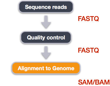
Image from “Data Wrangling and Processing for Genomics”
We perform read alignment or mapping to determine where in the genome our reads originated from. There are a number of tools to choose from and, while there is no gold standard, there are some tools that are better suited for particular NGS analyses. We will be using the STAR Aligner (STAR), which is a universal aligner for mapping sequences against a large reference genome.
The alignment process consists of two steps:
- Indexing the reference genome
- Aligning the reads to the reference genome
Setting up
Hands On: Index the reference genomeOur first step is to index the reference genome for use by STAR. Indexing allows the aligner to quickly find potential alignment sites for query sequences in a genome, which saves time during alignment. Indexing the reference only has to be run once. The only reason you would want to create a new index is if you are working with a different reference genome or you are using a different tool for alignment.
Code In: Indexing with `STAR`$ mkdir index $ STAR --runThreadN 16 --runMode genomeGenerate --genomeDir ~/index --genomeFastaFiles /import/14 --sjdbGTFfile /import/15 --sjdbOverhang 100 --genomeSAindexNbases 12While the index is created and saved in the index folder, you will see output that looks something like this:
Code OutSTAR version: 2.7.10b compiled: 2022-11-01T09:53:26-04:00 :/home/dobin/data/STAR/STARcode STAR.master/source Date Time ..... started STAR run Date Time ... starting to generate Genome files Date Time ..... processing annotations GTF Date Time ... starting to sort Suffix Array. This may take a long time... Date Time ... sorting Suffix Array chunks and saving them to disk...
Hands On: Align reads to reference genomeThe alignment process consists of choosing an appropriate reference genome to map our reads against and then deciding on an aligner. We will use the STAR algorithm as said.
An example of what a
STARcommand looks like is below. This command will not run, as we do not have the files:input_file_R1orinput_file_R2.$ STAR --genomeDir /index_folder --runThreadN 16 --readFilesIn /trimmedData/input_file_R1 /trimmedData/input_file_R2Have a look at the STAR manual, while we are running STAR with the default
parameters here, your use case might require a change of parameters. NOTE: Always read the manual page for any tool before using and make sure the options you use are appropriate for your data.
We are going to start by aligning the reads from just one of the samples in our dataset (GSM461177). After that, we will be iterating the following process on the second pair of our sample files (GSM461180).
Code In: Aligning with STAR$ STAR --genomeDir ~/index --runThreadN 16 -- readFilesIn /trimmedData/GSM461177_R1 /trimmedData/GSM461177_R2 --outFileNamePrefix GSM461177Code OutDate Time ..... started STAR run Date Time ..... loading genome Date Time ..... started mapping
SAM/BAM format
The SAM file, is a tab-delimited text file that contains information for each individual read and its alignment to the genome. While we do not have time to go into detail about the features of the SAM format, the paper by Heng Li et al. provides a lot more detail on the specification.
The compressed binary version of SAM is called a BAM file. We use this version to reduce size and to allow for indexing, which enables efficient random access of the data contained within the file.
The file begins with a header, which is optional for SAM files. The header is used to describe the source of data, reference sequence, method of alignment, etc., this will change depending on the aligner being used. Following the header is the alignment section. Each line that follows corresponds to alignment information for a single read. Each alignment line has 11 mandatory fields for essential mapping information and a variable number of other fields for aligner specific information. An example entry from a SAM file is displayed below with the different fields highlighted.
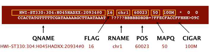
Image from Data Wrangling and Processing for Genomics
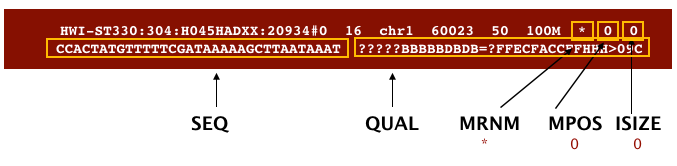
Image from “Data Wrangling and Processing for Genomics”
Hands On: SAM to BAMCode In: bashWe will convert the SAM file to BAM format using the
samtoolsprogram with theviewcommand and tell this command that the input is in SAM format (-S) and to output BAM format (-b). We will start with the first sample (GSM461177) and repeat the process with the second (GSM461180):$ samtools view -S -b GSM461177Aligned.out.sam > GSM461177Aligned.out.bamCode Out[samopen] SAM header is present: 1 sequences.
Hands On: Sort BAM file by coordinatesNext we sort the BAM file using the
sortcommand fromsamtools.-otells the command where to write the output.Code In: `sort` command$ samtools sort -o GSM461177Aligned.out.sorted.bam GSM461177Aligned.out.bamOur files are pretty small, so we will not see this output. If you run the workflow with larger files, you will see something like this:
Code Out[bam_sort_core] merging from 2 files...SAM/BAM files can be sorted in multiple ways, e.g. by location of alignment on the chromosome, by read name, etc. It is important to be aware that different alignment tools will output differently sorted SAM/BAM, and different downstream tools require differently sorted alignment files as input.
You can use samtools to learn more about this bam file as well.
Counting reads per genes
Time to tie things up! To compare the expression of single genes between different conditions (e.g. with or without PS depletion), an essential first step is to quantify the number of reads per gene, or more specifically the number of reads mapping to the exons of each gene.
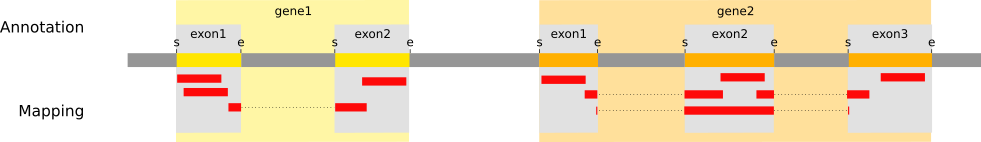 Open image in new tab
For the final step of this tutorial we will use featureCounts to count the number of reads per annotated gene.
Hands On: FeatureCountsThe main output of featureCounts is a table with the counts, i.e. the number of reads (or fragments in the case of paired-end reads) mapped to each gene (in rows, with their ID in the first column) in the provided annotation. FeatureCount generates also the feature length output datasets. Keep in mind that the “/import/7/” corresponds to D. melanogaster’s gene annotation file we imported in RStudio way back.
Code In: featureCounts$ featureCounts -a /import/7 -T 8 -o featurecounts.txt -p GSM461177Aligned.out.sorted.bam GSM461180Aligned.out.sorted.bamThe featurecounts.txt produced contains all the information needed for further downstream analysis of the sequences we aligned (e.g. Differential Expression).
You've Finished the Tutorial
Key points
Bioinformatic command line tools are collections of commands that can be used to carry out bioinformatic analyses.
To use most powerful bioinformatic tools, you will need to use the command line.
There a few basic steps to follow in order to process the RNA sequences
Quality control, trimming and alignment to reference genome are the first part of the RNA-seq downstream analysis
Frequently Asked Questions
Have questions about this tutorial? Have a look at the available FAQ pages and support channelsUseful literature
Further information, including links to documentation and original publications, regarding the tools, analysis techniques and the interpretation of results described in this tutorial can be found here.
References
- Brooks, A. N., L. Yang, M. O. Duff, K. D. Hansen, J. W. Park et al., 2011 Conservation of an RNA regulatory map between Drosophila and mammals. Genome Research 21: 193–202. https://www.ncbi.nlm.nih.gov/pmc/articles/PMC3032923/
- Marcel, M., 2011 Cutadapt removes adapter sequences from high-throughput sequencing reads. EMBnet.journal 17: 10–12. http://journal.embnet.org/index.php/embnetjournal/article/view/200
Feedback
Did you use this material as an instructor? Feel free to give us feedback on how it went.
Did you use this material as a learner or student? Click the form below to leave feedback.

Citing this Tutorial
- Sofoklis Keisaris, RNA-seq Alignment with STAR (Galaxy Training Materials). https://training.galaxyproject.org/training-material/topics/transcriptomics/tutorials/rna-seq-bash-star-align/tutorial.html Online; accessed TODAY
- Hiltemann, Saskia, Rasche, Helena et al., 2023 Galaxy Training: A Powerful Framework for Teaching! PLOS Computational Biology 10.1371/journal.pcbi.1010752
- Batut et al., 2018 Community-Driven Data Analysis Training for Biology Cell Systems 10.1016/j.cels.2018.05.012
@misc{transcriptomics-rna-seq-bash-star-align,
author = "Sofoklis Keisaris",
	title = "RNA-seq Alignment with STAR (Galaxy Training Materials)",
	year = "",
	month = "",
	day = "",
	url = "\url{https://training.galaxyproject.org/training-material/topics/transcriptomics/tutorials/rna-seq-bash-star-align/tutorial.html}",
	note = "[Online; accessed TODAY]"
}
@article{Hiltemann_2023,
	doi = {10.1371/journal.pcbi.1010752},
	url = {https://doi.org/10.1371%2Fjournal.pcbi.1010752},
	year = 2023,
	month = {jan},
	publisher = {Public Library of Science ({PLoS})},
	volume = {19},
	number = {1},
	pages = {e1010752},
	author = {Saskia Hiltemann and Helena Rasche and Simon Gladman and Hans-Rudolf Hotz and Delphine Larivi{\`{e}}re and Daniel Blankenberg and Pratik D. Jagtap and Thomas Wollmann and Anthony Bretaudeau and Nadia Gou{\'{e}} and Timothy J. Griffin and Coline Royaux and Yvan Le Bras and Subina Mehta and Anna Syme and Frederik Coppens and Bert Droesbeke and Nicola Soranzo and Wendi Bacon and Fotis Psomopoulos and Crist{\'{o}}bal Gallardo-Alba and John Davis and Melanie Christine Föll and Matthias Fahrner and Maria A. Doyle and Beatriz Serrano-Solano and Anne Claire Fouilloux and Peter van Heusden and Wolfgang Maier and Dave Clements and Florian Heyl and Björn Grüning and B{\'{e}}r{\'{e}}nice Batut and},
	editor = {Francis Ouellette},
	title = {Galaxy Training: A powerful framework for teaching!},
	journal = {PLoS Comput Biol}
}
Funding
These individuals or organisations provided funding support for the development of this resource
Congratulations on successfully completing this tutorial!