Quantification of single-molecule RNA fluorescence in situ hybridization (smFISH) in yeast cell lines

Author(s)	Riccardo Massei
Reviewers

Overview
Questions:

How do I analyze fluorescence markers in a 2D image?

How do I create labels from the detected bright spots?

How can I count the number of detected spots automatically?

Objectives:

Perform a 2D spots/blobs detection in an image fetched from IDR

Count the detected spots and blo

Requirements:

Introduction to Galaxy Analyses

tutorial Hands-on: FAIR Bioimage Metadata

tutorial Hands-on: REMBI - Recommended Metadata for Biological Images – metadata guidelines for bioimaging data

tutorial Hands-on: Introduction to Image Analysis using Galaxy

Time estimation: 30 minutes

Level: Introductory Introductory

Supporting Materials:

Workflows

instances Available on these Galaxies

Known Working

UseGalaxy.eu ✅ ⭐️

UseGalaxy.cz ✅

Published: Mar 20, 2025

Last modification: Mar 20, 2025

License: Tutorial Content is licensed under Creative Commons Attribution 4.0 International License. The GTN Framework is licensed under MIT

version Revision: 2

The objective is to detect multiple bright spots in an image using a basic computer vision and image processing technique for identification and localization of regions of high intensity within an image. These spots often correspond to features of interest, such as fluorescent markers in biological imaging. Such an approach can be beneficial in single-cell/single-molecule imaging experiments, such as RNA single-molecule fluorescence in situ hybridization (smFISH), as these experiments can resolve the spatial and temporal distribution of individual RNA molecules with high resolution.

In this tutorial, we will try to identify RNA molecules in yeast cell lines. However, such an approach can be re-used for the identification of any fluorescence spots in biological images!

Agenda

In this tutorial, we will deal with:

Get data from IDR

Improve image contrast

RNA spots detection

Convert spots coordinates to labels

Overlay labels to the original image

Create 2D spot detection workflow

Conclusion

Get data from IDR

The testing dataset for this tutorial can be obtained from the Image Data Repository (IDR). This dataset was published by Li et al. (2019) in Scientific Data.

In this publication, the authors used smFISH to quantify the kinetic expression of STL1 and CTT1 mRNAs in single Saccharomyces cerevisiae cells upon NaCl osmotic stress.

Let’s fetch this FAIR dataset using a Galaxy Tool! We will download the channel 5-TMR and selected the 10th z-stack for analysis.

Hands On: Download images from the IDR

If you are logged in, create a new history for this tutorial.

To create a new history simply click the new-history icon at the top of the history panel:

IDR Download tool with the following parameters:

“How would you like to specify the IDs of images to download?”: As text (comma-separated list of IDs or a valid IDR link)

“Image IDs to download”: 4496770

*“Which Images do you want to download”: Exported TIFF (single channel, single stack)

“Name of the channel to download”: 5-TMR

“z-plane of images to download”: 10

“Image frame to download”: 0

“Limit the download to a selected region of the image?”: No, download the entire image plane

“Skip failed retrievals?”: No

“Download images in a tarball?”: No

Rename galaxy-pencil the generated file to RNA_input.

Improve image contrast

When inspecting the image visually, we get the impression that the image is entirely black:

It’s not the best quality for a first visual inspection!

As described in the Galaxy Imaging Introduction Tutorial, the original image is 16-bit and the intensity values are spread over a very small fraction of the range of intensity values that can be represented using 16 bits.

Therefore, for improved visibility the intensity histogram of the image can be normalized first.

We will normalize the histogram to improve the contrast. We do this using a Contrast Limited Adaptive Histogram Equalization (CLAHE) approach.

Hands On: Normalize Histogram

Perform histogram equalization ( Galaxy version 0.18.1+galaxy0) with the following parameters to normalize the histogram of the image:

param-file “Input image”: RNA_input.tif file

“Histogram equalization algorithm”: CLAHE

Rename galaxy-pencil the generated file to RNA_input_normalized.

Click on the visualise icon galaxy-visualise of the file to visually inspect the image using the Tiff Viewer visualization plugin.

Your image should now look a bit brighter:

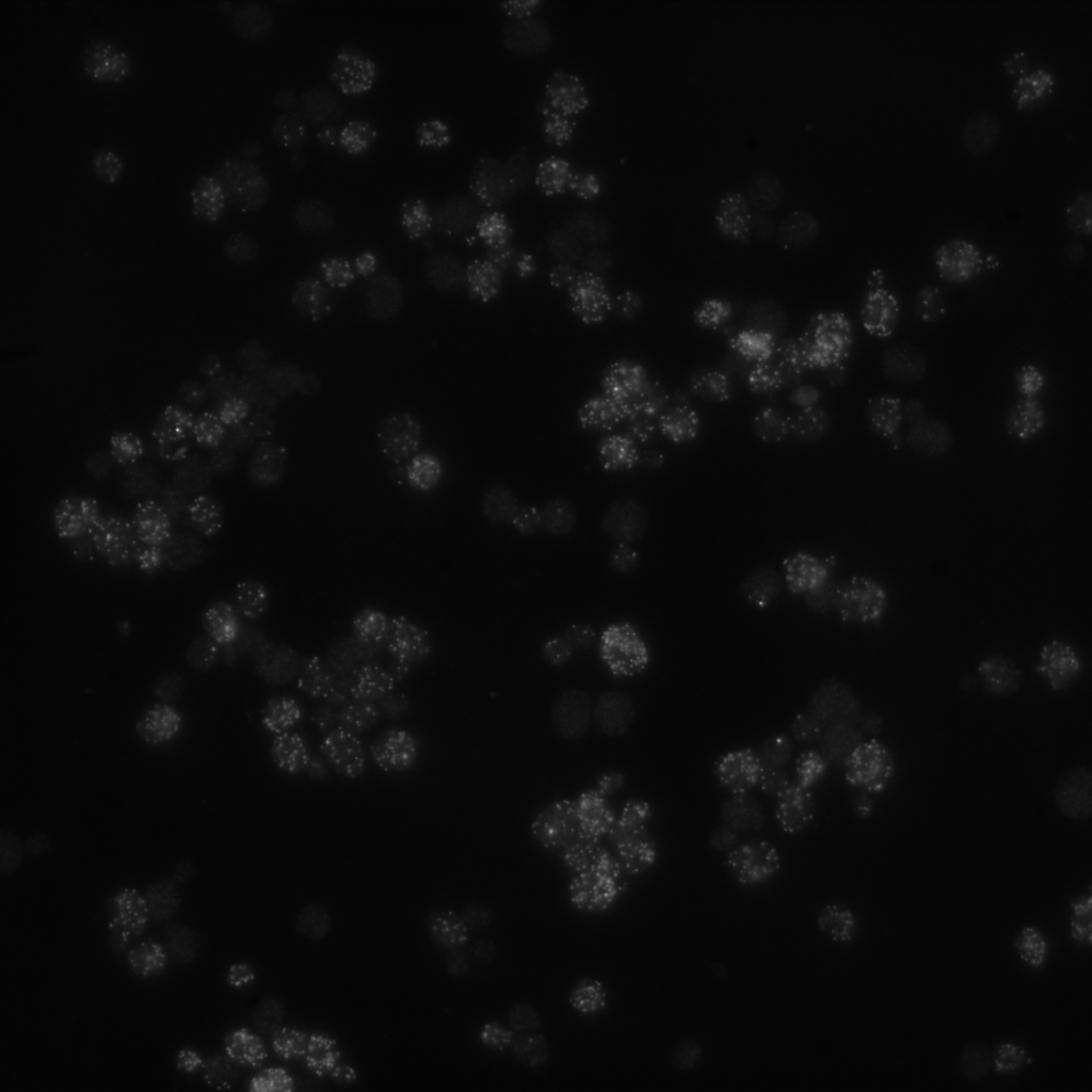
We can now clearly make out the presence of many RNA spots!

RNA spots detection

We can now try to detect blobs and measure their intensity… Let’s run a specific tool for this!

Hands On: Perform 2-D spot detection

Perform 2-D spot detection ( Galaxy version 0.1+galaxy0) with the following parameters to detect the 2D spots:

param-file “Intensity image or a stack of images”: RNA_input_normalized.tif file

“Starting time point (1 for the first frame of the stack) “: 1

“Ending time point (0 for the last frame of the stack)”: 0

“Detection filter”: Laplacian of Gaussian

“Minimum scale”: 1

“Maximum scale”: 2

“Minimum filter response (absolute)”: 0.25

“Minimum filter response (relative)”: 0

“Image boundary”: 10

Rename galaxy-pencil the generated file to RNA_spot_detected.

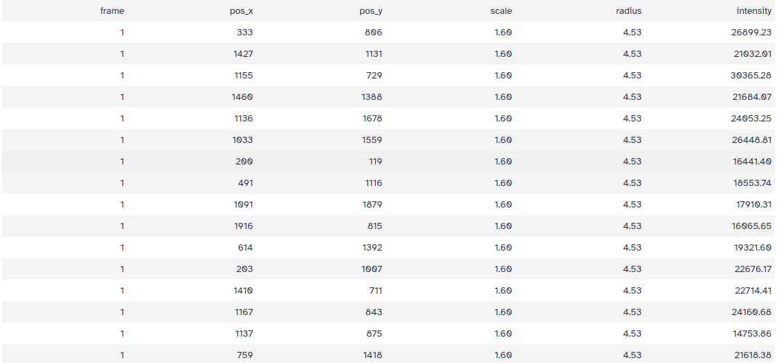
The tool produces a TSV file containing all detections, with the following columns:

frame: The frame of the image stack
pos_x: The horizontal coordinate of the detection
pos_y: The vertical coordinate of the detection
scale: The scale at which the detection was found
radius: The radius of the detected spot
intensity: The mean intensity of the spot

The TSV output will have 1649 lines, meaning 1649 spots detected!

Convert spots coordinates to labels

Let’s try now to visualize our results! The first step is to create a label map from the TSV file… This can be nicely done by converting the point coordinates to a label map and we have a tool for it!

Please notice that the width and height of the image are necessary inputs to corretly overlay the label map in the next step! You can get these info by running the “Show image info” tool on the original image!

Hands On: Create the label map from the points coordinates

Convert point coordinates to label map ( Galaxy version 0.4+galaxy0) with the following parameters to detect the 2D spots:

param-file “Tabular list of points”: RNA_spot_detected.tsv file

“Width of output image”: 2048

“Height of output image “: 2048

“Tabular list of points has header”: Yes

“Swap X and Y coordinates”: No

“Produce binary image”: No

Rename galaxy-pencil the generated file to RNA_labels.

Click on the visualise icon galaxy-visualise of the file to visually inspect the image using the Tiff Viewer visualization plugin.

A label image will be created… If you want to visualize the labels, you can run again the normalize histogram step:

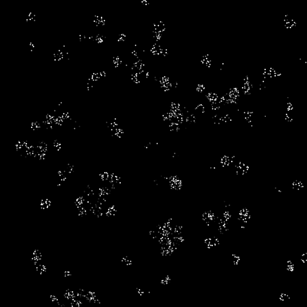
but this is not necessary for the next and final step: overlay the label to the original image!

Overlay labels to the original image

Results can be overlayed with the original image.

Hands On: Segment image

Overlay images ( Galaxy version 0.0.4+galaxy4) with the following parameters to convert the image to PNG:

“Type of the overlay”: Segmentation contours over image

param-file “Intensity image”: RNA_input_normalized.tif file

param-file “Label map”: RNA_labels.tif file (output of Convert binary image to label map ( Galaxy version 0.5+galaxy0))

“Contour thickness”: 1

“Contour color”: red

“Show labels”: No

“Label color”: yellow

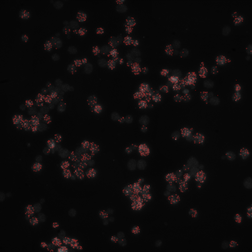
Final result should look like this:

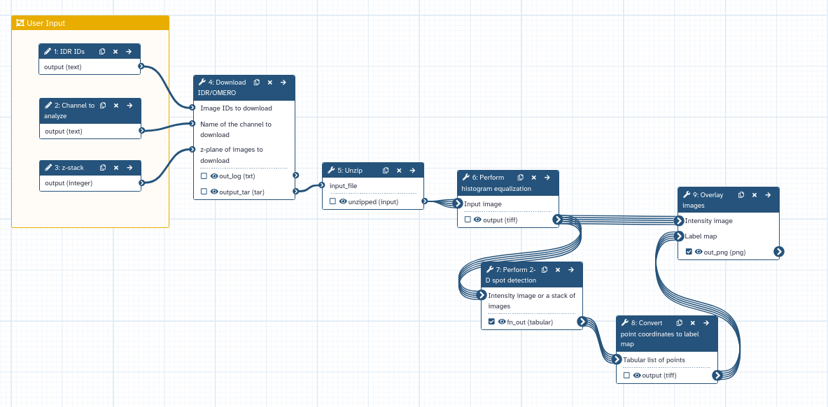
Create 2D spot detection workflow

The full workflow can now be created!

Since you are probably going to run it on several images fetched from IDR we suggest changing the setting of the IDR Download tool by downloading imaging in a tarball:

Hands On: Create the workflow for 2D spot detection

Name it “2D_spot_detection”.

Change “Download images in a tarball?”: Yes in the IDR Download tool tool

Include the Unzip ( Galaxy version 6.0+galaxy0)

Connect the output of param-file 4: Download IDR/OMERO to the “input_file” input of tool 5: Unzip.

Connect the output of param-file 4: Unzip to the “Input Image” input of tool 6: Perform histogram equalization.

Edit the workflow you just created:

Select “Input dataset” from the list of tools. The step param-file 1: Input Dataset appears.

Select “Text Input” from the list of tools. The step param-file 2: Text Input appears.

Select “Integer Input” from the list of tools. The step param-file 3: Integer Input appears.

Change the “Label” of param-file 1: Input Dataset to IDR IDs.

Change the “Label” of param-file 2: Text Input to Channel selection.

Change the “Label” of param-file 3: Integer Input to z-stack selection.

Connect the output of param-file 1: Input Dataset to the “Image IDs to download” input of tool 4: Download IDR/OMERO.

Connect the output of param-file 2: Text Input to the “Name of the channel to download” input of tool 4: Download IDR/OMERO.

Connect the output of param-file 3: Integer Input to the “z-plane of images to download” input of tool 4: Download IDR/OMERO.

Mark the results of tool 7: Perform 2-D spot detection and tool 9: Overlay images as the primary outputs of the workflow (by clicking on the checkboxes of the outputs).

The final workflow should look like this:

Conclusion

In this exercise, you imported images into Galaxy from IDR, detect RNA single molecules using the 2D spot detection tool and visualize them on the original intensity image. Finally, you created a reusable workflow which can be used on a tarball of IDR images.

You've Finished the Tutorial

Key points

Fluorescent markers can be detected using Galaxy

Objects can be automatically counted and the intensity range can be plotted

Frequently Asked Questions

Have questions about this tutorial? Have a look at the available FAQ pages and support channels

Useful literature

Further information, including links to documentation and original publications, regarding the tools, analysis techniques and the interpretation of results described in this tutorial can be found here.

Feedback

Did you use this material as an instructor? Feel free to give us feedback on how it went.
Did you use this material as a learner or student? Click the form below to leave feedback.

Citing this Tutorial

Riccardo Massei, Quantification of single-molecule RNA fluorescence in situ hybridization (smFISH) in yeast cell lines (Galaxy Training Materials). https://training.galaxyproject.org/training-material/topics/imaging/tutorials/2D-spot-detection/tutorial.html Online; accessed TODAY
Hiltemann, Saskia, Rasche, Helena et al., 2023 Galaxy Training: A Powerful Framework for Teaching! PLOS Computational Biology 10.1371/journal.pcbi.1010752
Batut et al., 2018 Community-Driven Data Analysis Training for Biology Cell Systems 10.1016/j.cels.2018.05.012

@misc{imaging-2D-spot-detection,
author = "Riccardo Massei",
	title = "Quantification of single-molecule RNA fluorescence in situ hybridization (smFISH) in yeast cell lines (Galaxy Training Materials)",
	year = "",
	month = "",
	day = "",
	url = "\url{https://training.galaxyproject.org/training-material/topics/imaging/tutorials/2D-spot-detection/tutorial.html}",
	note = "[Online; accessed TODAY]"
}
@article{Hiltemann_2023,
	doi = {10.1371/journal.pcbi.1010752},
	url = {https://doi.org/10.1371%2Fjournal.pcbi.1010752},
	year = 2023,
	month = {jan},
	publisher = {Public Library of Science ({PLoS})},
	volume = {19},
	number = {1},
	pages = {e1010752},
	author = {Saskia Hiltemann and Helena Rasche and Simon Gladman and Hans-Rudolf Hotz and Delphine Larivi{\`{e}}re and Daniel Blankenberg and Pratik D. Jagtap and Thomas Wollmann and Anthony Bretaudeau and Nadia Gou{\'{e}} and Timothy J. Griffin and Coline Royaux and Yvan Le Bras and Subina Mehta and Anna Syme and Frederik Coppens and Bert Droesbeke and Nicola Soranzo and Wendi Bacon and Fotis Psomopoulos and Crist{\'{o}}bal Gallardo-Alba and John Davis and Melanie Christine Föll and Matthias Fahrner and Maria A. Doyle and Beatriz Serrano-Solano and Anne Claire Fouilloux and Peter van Heusden and Wolfgang Maier and Dave Clements and Florian Heyl and Björn Grüning and B{\'{e}}r{\'{e}}nice Batut and},
	editor = {Francis Ouellette},
	title = {Galaxy Training: A powerful framework for teaching!},
	journal = {PLoS Comput Biol}
}

                   

Funding

These individuals or organisations provided funding support for the development of this resource

NFDI4Bioimage

DFG

Congratulations on successfully completing this tutorial!

You can use Ephemeris's shed-tools install command to install the tools used in this tutorial.

shed-tools install [-g GALAXY] [-a API_KEY] -t <(curl https://training.galaxyproject.org/training-material/api/topics/imaging/tutorials/2D-spot-detection/tutorial.json | jq .admin_install_yaml -r)

Alternatively you can copy and paste the following YAML

---
install_tool_dependencies: true
install_repository_dependencies: true
install_resolver_dependencies: true
tools:
- name: 2d_histogram_equalization
  owner: imgteam
  revisions: b1c2c210813c
  tool_panel_section_label: Imaging
  tool_shed_url: https://toolshed.g2.bx.psu.edu/
- name: binary2labelimage
  owner: imgteam
  revisions: 984358e43242
  tool_panel_section_label: Imaging
  tool_shed_url: https://toolshed.g2.bx.psu.edu/
- name: overlay_images
  owner: imgteam
  revisions: ca362a9bfa20
  tool_panel_section_label: Imaging
  tool_shed_url: https://toolshed.g2.bx.psu.edu/
- name: points2labelimage
  owner: imgteam
  revisions: de611b3b5ae8
  tool_panel_section_label: Imaging
  tool_shed_url: https://toolshed.g2.bx.psu.edu/
- name: spot_detection_2d
  owner: imgteam
  revisions: e8c9e104e109
  tool_panel_section_label: Imaging
  tool_shed_url: https://toolshed.g2.bx.psu.edu/
- name: unzip
  owner: imgteam
  revisions: 57f0914ddb7b
  tool_panel_section_label: Collection Operations
  tool_shed_url: https://toolshed.g2.bx.psu.edu/
- name: idr_download_by_ids
  owner: iuc
  revisions: f92941d1a85e
  tool_panel_section_label: Imaging
  tool_shed_url: https://toolshed.g2.bx.psu.edu/

No feedback has been recieved yet for this training. Be the first one by filling in the feedback form.