nb2workflow: Generating Galaxy Tools From Jupyter Notebooks
| Author(s) |
|
| Editor(s) |
|
| Reviewers |
|
OverviewQuestions:
Objectives:
How can new-to-Galaxy developers convert functioning Jupyter Notebooks into Galaxy tools?
How are the inputs and outputs defined?
How are the tool dependencies provided?
Requirements:
Learn why you might want to use the nb2galaxy.
Install the package and explore the provided example notebooks.
Modify the examples and regenerate the tools to check the effects.
Create new Galaxy tools from your own Jupyter Notebooks.
- slides Slides: A short introduction to Galaxy
- tutorial Hands-on: A short introduction to Galaxy
- tutorial Hands-on: Galaxy Basics for everyone
- slides Slides: Tool development and integration into Galaxy
- tutorial Hands-on: Tool development and integration into Galaxy
Time estimation: 1 hourSupporting Materials:
Published: Dec 4, 2025Last modification: Dec 4, 2025License: Tutorial Content is licensed under Creative Commons Attribution 4.0 International License. The GTN Framework is licensed under MITpurl PURL: https://gxy.io/GTN:T00567version Revision: 1
With the advance of python and Jupyter Notebooks, many astronomers have started using them for their data analysis pipelines. In response, members of the astronomy and data science communities have developed nb2galaxy – a module of the nb2workflow library – that allows for a quick and easy conversion of Jupyter Notebooks into Galaxy tools. While originally motivated by astronomical use cases, the tool is broadly applicable. This tutorial is therefore aimed at developers and researchers across disciplines who are interested in Galaxy.
Agenda
Convert an example Jupyter notebook into a Galaxy tool
This tutorial starts with the setup of the required enviornment and a very basic Jupyter Notebook. Afterwards, each section introduces one or more concepts related to the conversion. The tutorial ends with a more complex example of inputs and outputs.
It is important to mention that the end result of this tutorial is a folder with a .xml file that describes the tool and other required files for the tool to function. In order for the tool to be on the UseGalaxy platform, one needs to publish the resulting folder on toolshed and UseGalaxy.
Environment Setup
This tutorial uses the JupyterLab interface to edit notebooks, but any Jupyter-compatible editor (such as VS Code) will work just as well.
The example notebook relies only on the numpy and matplotlib libraries. Two additional packages are required: nb2workflow that provides the nb2galaxy conversion module and planemo which is used to test and preview the generated Galaxy tool locally.
To create a virtual environment with all required packages:
mkdir nb2galaxy-example
cd nb2galaxy-example
python -m venv .venv
source .venv/bin/activate
pip install jupyterlab numpy matplotlib nb2workflow[galaxy] planemo
The initial notebook, that is used to plot a function $y=x^p$ in a given range, can be downloaded from:
wget https://raw.githubusercontent.com/esg-epfl-apc/nb2galaxy-example-repo/refs/tags/step-0/example_nb2workflow.ipynb
Open Jupyter lab to preview the notebook
jupyter lab
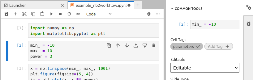
Tagging Inputs and Outputs
Since nb2galaxy recognizes cell tags following the Papermill convention, one needs to create dedicated cells for the input and output of the notebook and then tag them accordingly. In the current example, the second cell is tagged as “parameters” and contains the input values:
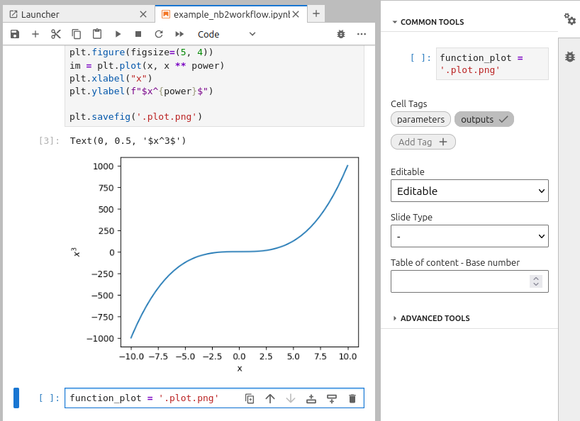
In order to obtain the output, one must save the figure to a file and provide its path in a new cell tagged as “outputs”:
Defining Dependencies
The automatic conversion of the notebook to a Galaxy tool requires an explicit definition of the dependencies. As long as Galaxy uses conda to install tool dependencies, the preferred way is to create an environment.yml file, even though nb2galaxy supports both environment.yml and requirements.txt. Here’s an example environment.yml:
name: nb2galaxy-example
channels:
  - conda-forge
dependencies:
  - numpy
  - matplotlib
When both environment.yml and requirements.txt are present, nb2galaxy attempts to reconcile them using Conda. First, each package from requirements.txt is searched by conda. If the package with the same name exists in the configured conda channels (only conda-forge by default), it is included in the final list of packages for reconciliation. Otherwise, the package is ignored, and a comment is added to the generated tool represented as an XML file.
In the end, all dependencies are resolved together to obtain fixed versions of the required packages that are written in the tool’s XML file.
Notebook to Galaxy tool conversion
At this stage, one can create a very simple Galaxy tool using nb2galaxy CLI:
nb2galaxy --environment_yml environment.yml example_nb2workflow.ipynb ./tooldir
This creates the ./tooldir folder that contains a tool description .xml file and a python script file:
tooldir/
├── example_nb2workflow.py
└── example.xml

1 directory, 2 files
The minimal tool created from the notebook is ready. One can preview it locally with planemo:
planemo serve ./tooldir
Improving the tool
In order to publish a tool on the UseGalaxy platform, the tool needs to pass the planemo linting tests. Currently, the example tool does not pass the tests:
$ planemo lint ./tooldir/
Linting tool /home/dsavchenko/Projects/ESG/nb2galaxy-example-repo/tooldir/example.xml
.. CHECK (TestsNoValid): 1 test(s) found.
.. INFO (OutputsNumber): 1 outputs found.
.. INFO (InputsNum): Found 3 input parameters.
.. WARNING (HelpMissing): No help section found, consider adding a help section to your tool.
.. CHECK (ToolIDValid): Tool defines an id [example].
.. CHECK (ToolNameValid): Tool defines a name [example].
.. CHECK (ToolProfileValid): Tool specifies profile version [24.0].
.. CHECK (ToolVersionValid): Tool defines a version [0.1.0+galaxy0].
.. INFO (CommandInfo): Tool contains a command.
.. WARNING (CitationsMissing): No citations found, consider adding citations to your tool.
Failed linting
The tool requires a “help section” and citations. nb2galaxy can extract the “help section” from either .rst or .md files and citations from a BibTex .bib file.
Let us create a markdown file galaxy_help.md with the following help text:
This tool is a simple example, automatically created from a Jupyter notebook using `nb2galaxy`.
and a CITATION.bib file:
@software{nb2galaxy-example,
  author = {Variu, Andrei and Savchenko, Denys},
  title = "Example of nb2galaxy",
  url = {https://github.com/esg-epfl-apc/nb2galaxy-example-repo},
  year = {2025}
}
Finally, by regenerating the tool
nb2galaxy --environment_yml environment.yml --citations_bibfile CITATION.bib --help_file galaxy_help.md example_nb2workflow.ipynb tooldir
the planemo lint tests should pass.
Annotating input parameters
By default, nb2galaxy assumes all input parameters are of type Integer. Even though one can change the default configuration, one can explicitly provide parameter types using semantic annotations or python type annotations.
In this tutorial, we focus on semantic annotations because they allow for additional options. Out of the box, the conversion module uses the astronomy-specific ontology, described at https://odahub.io/ontology/, although a different ontology can be specified via a CLI option.
Semantic annotations are added as comments following the parameter assignment. The syntax follows the truncated Turtle format, where the input parameter is implicitly considered the subject and the a predicate is optional.
In the current example:
min_ = -10 # http://odahub.io/ontology#Float
max_ = 10 # http://odahub.io/ontology#Float
power = 3 # http://odahub.io/ontology#Integer
To improve readability, one can use the oda: prefix as a shorthand for http://odahub.io/ontology#, similar to how rdfs: shortens http://www.w3.org/2000/01/rdf-schema#. With this abbreviation, the annotations become:
min_ = -10 # oda:Float
max_ = 10 # oda:Float
power = 3 # oda:Integer
Automatically, the variable names are used as labels in the tool interface. However, one can provide custom labels using semantic annotations, allowing for more user-friendly descriptions to be displayed:
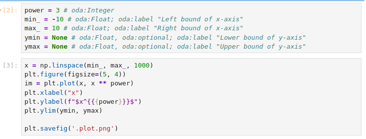
min_ = -10 # oda:Float; oda:label "Left bound of x-axis"
max_ = 10 # oda:Float; oda:label "Right bound of x-axis"
power = 3 # oda:Integer
Let us modify the notebook to add optional y-axis bounds:
The resulting Jupyter notebook is available at https://github.com/esg-epfl-apc/nb2galaxy-example-repo/blob/step-2/example_nb2workflow.ipynb.
By recreating the tool
nb2galaxy --environment_yml environment.yml --citations_bibfile CITATION.bib --help_file galaxy_help.md example_nb2workflow.ipynb tooldir
the planemo lint checks should pass and one can locally test the tool using planemo serve as before.
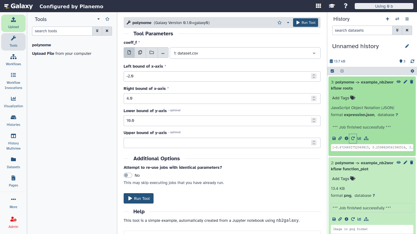
Working with Input Datasets
Jupyter Notebooks often use datasets as inputs. In this section, we explain how to modify the previous notebook to accept a file as input. Specifically, the updated notebook should read polynomial coefficients from a .csv file, compute the roots and generate a plot of the corresponding polynomial function.
Firstly, create an input file, dataset.csv, which allows to run the notebook. This file also serves as test data for the generated tool.
-1.2,3.2,6,-2.1
Furthermore, replace the power input parameter from the notebook with:
coeff_f = 'dataset.csv' # oda:POSIXPath
where every parameter annotated with http://odahub.io/oontology#POSIXPath or its subclasses is treated as an input dataset.
Read the polynomial coefficients from the input .csv file and use the numpy.polynomial.Polynomial function:
coeff = np.genfromtxt(coeff_f, delimiter=',')
p = Polynomial(coeff)
Update the plot method invocation in the next cell
x = np.linspace(min_, max_, 1000)
plt.figure(figsize=(5, 4))
im = plt.plot(x, p(x), label=f"{p}")
plt.xlabel("x")
plt.legend()
plt.ylim(ymin, ymax)

plt.savefig('.plot.png')
and add an additional output for the polynomial roots
function_plot = '.plot.png'
roots = list(p.roots())
You can consult the resulting notebook at https://github.com/esg-epfl-apc/nb2galaxy-example-repo/blob/step-3/example_nb2workflow.ipynb.
Afterwards, cleanup the tool directory rm -rf tooldir and regenerate the tool using the new name polynome:
nb2galaxy --name polynome --environment_yml environment.yml --citations_bibfile CITATION.bib --help_file galaxy_help.md example_nb2workflow.ipynb tooldir
Finally, lint the tool with planemo lint tooldir and preview it with planemo serve tooldir. The tool should accept a dataset as input and generate two outputs: a plot of the polynomial function and a JSON expression with the list of roots of the corresponding polynomial.
Acknowledgements
This tutorial is part of EuroScienceGateway project.
Parts of nb2workflow library is developed and tested with support from OSCARS, ACME,
AstroORDAS Explore and
AstroORDAS Establish
projects.
You've Finished the Tutorial
Key points
The nb2galaxy module of the nb2workflow library is an automated Galaxy tool generator for scientists and developers who routinely write Jupyter Notebooks.
nb2workflow is a Python package that can be easily installed via pip.
Once a Jupyter Notebook is functional, only a clear separation and definition of the inputs and outputs - along with appropriate annotations and tags - is needed for conversion.
The conversion module accepts additional files (e.g., help text, citations, environment specifications) to ensure the generated tool passes planemo lint checks.
Frequently Asked Questions
Have questions about this tutorial? Have a look at the available FAQ pages and support channelsFeedback
Did you use this material as an instructor? Feel free to give us feedback on how it went.
Did you use this material as a learner or student? Click the form below to leave feedback.

Citing this Tutorial
- Denys Savchenko, Andrei Variu, nb2workflow: Generating Galaxy Tools From Jupyter Notebooks (Galaxy Training Materials). https://training.galaxyproject.org/training-material/topics/dev/tutorials/tool-from-notebook/tutorial.html Online; accessed TODAY
- Hiltemann, Saskia, Rasche, Helena et al., 2023 Galaxy Training: A Powerful Framework for Teaching! PLOS Computational Biology 10.1371/journal.pcbi.1010752
- Batut et al., 2018 Community-Driven Data Analysis Training for Biology Cell Systems 10.1016/j.cels.2018.05.012
@misc{dev-tool-from-notebook,
author = "Denys Savchenko and Andrei Variu",
	title = "nb2workflow: Generating Galaxy Tools From Jupyter Notebooks (Galaxy Training Materials)",
	year = "",
	month = "",
	day = "",
	url = "\url{https://training.galaxyproject.org/training-material/topics/dev/tutorials/tool-from-notebook/tutorial.html}",
	note = "[Online; accessed TODAY]"
}
@article{Hiltemann_2023,
	doi = {10.1371/journal.pcbi.1010752},
	url = {https://doi.org/10.1371%2Fjournal.pcbi.1010752},
	year = 2023,
	month = {jan},
	publisher = {Public Library of Science ({PLoS})},
	volume = {19},
	number = {1},
	pages = {e1010752},
	author = {Saskia Hiltemann and Helena Rasche and Simon Gladman and Hans-Rudolf Hotz and Delphine Larivi{\`{e}}re and Daniel Blankenberg and Pratik D. Jagtap and Thomas Wollmann and Anthony Bretaudeau and Nadia Gou{\'{e}} and Timothy J. Griffin and Coline Royaux and Yvan Le Bras and Subina Mehta and Anna Syme and Frederik Coppens and Bert Droesbeke and Nicola Soranzo and Wendi Bacon and Fotis Psomopoulos and Crist{\'{o}}bal Gallardo-Alba and John Davis and Melanie Christine Föll and Matthias Fahrner and Maria A. Doyle and Beatriz Serrano-Solano and Anne Claire Fouilloux and Peter van Heusden and Wolfgang Maier and Dave Clements and Florian Heyl and Björn Grüning and B{\'{e}}r{\'{e}}nice Batut and},
	editor = {Francis Ouellette},
	title = {Galaxy Training: A powerful framework for teaching!},
	journal = {PLoS Comput Biol}
}
Funding
These individuals or organisations provided funding support for the development of this resource