ProteoRE Galaxy instance provides necessary tools to execute a whole annotation pipeline of a protein list identified by LC-MS/MS experiments. This activity introduces these tools and guides you through a simple pipeline using some example datasets based on the study entitled “Proteomic characterization of human exhaled breath condensate” Lacombe et al. 2018. The goal of this study was to identify proteins secreted in the respiratory tract (lung, bronchi). Samples were obtained non-invasively by condensation of exhaled air that contains submicron droplets of airway lining fluid. Two pooled samples of EBC, each obtained from 10 healthy donors, were processed. Two ‘technical’ control samples were processed in parallel to the pooled samples to correct for exogenous protein contamination. A total of 229 unique proteins were identified in EBC among which 153 proteins were detected in both EBC pooled samples. A detailed bioinformatics analysis of these 153 proteins showed that most of the proteins identified corresponded to proteins secreted in the respiratory tract (lung, bronchi).

Agenda

1. Get Input Datasets
2. Filtering out technical contaminants
3. Check for the presence of biological contaminants
4. Functional annotation of the EBC proteome (enrichment analysis)
5. Visualize EBC proteome on biological pathways (using Reactome)
6. Comparison with other proteomic datasets from previous studies
7. Conclusion

Get Input Datasets

For this tutorial, we will use 3 datasets: the list of proteins identified by LC-MS/MS in the exhaled breath condensate (EBC) from Lacombe et al. 2018 and two others EBC proteomes previously published (Muccilli et al. 2015 and Bredberg et al. 2011). These datasets are available from Zenodo here.

Hands-on: Data upload

1. Create a new history for this tutorial and give it a name

   Tip: Creating a new history

   To create a new history simply click the new-history icon at the top of the history panel:

   

2. Import the files from Zenodo or from the shared data library (ask your instructors).

   https://zenodo.org/record/3405119/files/Lacombe_2018.txt
   https://zenodo.org/record/3405119/files/Bredberg.txt
   https://zenodo.org/record/3405119/files/Mucilli.txt
   

   Tip: Importing via links

   • Copy the link location

   • Click galaxy-upload Upload Data at the top of the tool panel

   • Select galaxy-wf-edit Paste/Fetch Data

   • Paste the link(s) into the text field

   • Press Start

   • Close the window

   Tip: Importing data from a data library

   As an alternative to uploading the data from a URL or your computer, the files may also have been made available from a shared data library:

   1. Go into Data (top panel) then Data libraries
   2. Navigate to the correct folder as indicated by your instructor.
      • On most Galaxies tutorial data will be provided in a folder named GTN - Material –> Topic Name -> Tutorial Name.
   3. Select the desired files
   4. Click on Add to History galaxy-dropdown near the top and select as Datasets from the dropdown menu

   5. In the pop-up window, choose

      • “Select history”: the history you want to import the data to (or create a new one)
   6. Click on Import

Filtering out technical contaminants

A group of 10 proteins were identified in both “technical” control samples with an enrichment in EBC samples below a fixed threshold. These proteins were thus considered to be technical contaminants (see list of proteins in Table 4 in Lacombe et al. 2018) and have to be removed from the initial dataset.

Hands-on: Remove the contaminants

1. Filter by keywords and/or numerical value tool with the following parameters:
   • param-file “Input file”: Lacombe_2018.txt
   • “Operation”: Discard
   • param-repeat “Insert Filter by keywords”
     • “Column number on which to apply the filter”: c1
     • “Search for exact match ?”: No
     • “Enter keywords”: copy/paste
       • “Copy/paste keywords to find”: P04264 P35908 P13645 Q5D862 Q5T749 Q8IW75 P81605 P22531 P59666 P78386

   Comment: Outputs

   • Filtered_Lacombe_2018.txt - Discarded_lines: output list with the ten proteins (contaminants) removed from the original dataset (10 proteins)
   • Filtered_Lacombe_2018.txt: output contains the remaining proteins that will be considered for further analysis (151 proteins)

Check for the presence of biological contaminants

As EBC samples are obtained from air exhaled through the oral cavity, and even though the RTube collection device contained a saliva trap to separate saliva from the exhaled breath, contamination with salivary proteins had to be assessed. We decided to check the expression pattern for each protein of the “core” EBC proteome using the The Human Protein Atlas (HPA, Uhlén et al. 2005). As HPA is indexed by Ensembl gene identifier (ENSG) we first need to convert Uniprot ID to Ensembl gene (ENSG). Secondly, check for proteins which are highly expressed in the salivary glands as reported by HPA, then in a third step, we filter out these proteins.

Hands-on: Convert Uniprot ID to Ensembl gene ID

1. ID Converter tool with the following parameters:
   • “Enter IDs”: Input file containing IDs
     • param-file “Select your file”: Filtered_Lacombe_2018.txt output from Filter by keywords tool
   • “Column number of IDs to map”: c1
   • “Species”: Human (Homo sapiens)
     • “Type/source of IDs”: Uniprot accession number (e.g. P31946)
     • “Target type of IDs you would like to map to”:
       • param-check Ensembl gene ID (e.g. ENSG00000166913)

   Comment: Output

   In the output file, a new column which contains Ensembl IDs was added (at the end)

Hands-on: Check for proteins highly expressed in salivary glands

1. Add expression data tool with the following parameters:
   • “Enter your IDs”: Input file containing your IDs
   • param-file “Select your file”: ID Converter on data .. from ID Converter tool
   • “Column IDs”: c4 (column containing Ensembl IDs)
   • “Does file contain header”: Yes
   • “Select informareactometion to add to your list”:
     • param-check Gene name
     • param-check Gene description
     • param-check RNA tissue category (according to HPA)
     • param-check RNA tissue specificity abundance in "Transcript Per Million

   Comment: Outputs

   In the output file, four columns were added (5, 6, 7 and 8) corresponding to the retrieved information from HPA.

Examine the output table. Note that in the last column of the list (column 8), we see that AMY1B, CALML5, PIP, ZG16B, CST4, MUC7, CST1 and CST2 have been reported as highly enriched in salivary gland with elevated RNA transcript specific Transcript Per Million (TPM) value for each, suggesting that these proteins may come from the saliva and not from the exhaled breath condensate. We will remove these biological contaminants from our initial protein set.

[..]
P04745  Alpha-amylase           1  23  ENSG00000174876  AMY1B  Amylase, alpha 1B (salivary) Tissue enriched   salivary gland: 1847.5
[..]
Q9NZT1  Calmodulin-like protein 5  8  ENSG00000178372   CALML5 Calmodulin-like 5            Group enriched    salivary gland: 262.7;skin: 651.2
[..]

In the next step, we will filter the data to remove these biological contaminants (i.e. proteins highly expressed in salivary glands) by filtering out the lines that contain the word salivary in the column of RNA transcript specific TPM.

Hands-on: Filter the data to remove the biological contaminants

1. Filter by keywords and/or numerical value tool with the following parameters:
   • param-file “Input file”: Add expression data on data .. from Add expression data tool
   • “Operation”: Discard
   • param-repeat “Insert Filter by keywords”
     • “Column number on which to apply the filter” : c8 (column with RNA transcript specific TPM)
     • *“Search for exact match ?” : No
     • “Enter keywords”: copy/paste
       • “Copy/paste keyword to fine”: salivary

   Comment: Outputs

   Two output files are created:

   • Filtered Add expression data on data .. - Discarded lines (12 proteins)
   • FilteredAdd expression data on data .. (157 proteins)

Tip: Using genes instead of keywords

Note also that a list of “gene” may have been entered (selected on the basis of their TPM value) applied to column 5 instead of the keywords “salivary” to column 8, as it has been done in Lacombe et al. 2018.

Functional annotation of the EBC proteome (enrichment analysis)

The resulting list of 157 proteins identified in the two pooled EBC samples (excluding the 10 contaminants proteins) is now submitted to Gene Ontology (GO)-term enrichment analysis to determine functions that were significantly enriched in our EBC proteomic dataset. To do so, we’ll use the ClusterProfiler tool (based on the R package clusterProfiler) for functional annotation. Now we can perform the GO terms analysis. Input list is the EBC proteome to be analyzed after technical and biological contaminants removal, which is the output of biological contaminants filter step.

Hands-on: GO terms analysis

1. GO terms classification and enrichment analysis tool with the following parameters:
   • “Enter your IDs”: Input file containing your IDs
   • param-file “Choose a file that contains your list of IDs”: Filtered_Add expression data on data .. from Filter by keywords tool
   • “Column number of IDs”: c1
   • “Select type/source of IDs”: UniProt accession number (e.g.:P31946)
   • “Species”: Homo sapiens
   • “Select GO terms category”:
     • param-check Cellular Component
     • param-check Biological process
     • param-check Molecular Function
   • “Perform GO categories representation analysis?”: Yes
   • “Ontology level”: 3
   • “Perform GO categories enrichment analysis?”: Yes
     • “Define your own background IDs?”: No
       • “Graphical display”:
         • param-check dot-plot

Comment: Output

Results created in History panel are the following:

• Cluster profiler
• ClusterProfiler diagram outputs (collection dataset of all graphical outputs)
• ClusterProfiler text files (collection dataset of all text files)

The suffix “GGO” (GroupGO) corresponds to the results “GO categories representation analysis” option (performs a gene/protein classification based on GO distribution at a specific level). The suffix “EGO” (EnrichGO) corresponds to the results from the enrichment analysis. Two types of graphical output are provided either in the form of bar-plot or dot-plot.

Visualize EBC proteome on biological pathways (using Reactome)

The 157 proteins identified in EBC samples are now mapped to biological pathways and visualized via the web service of Reactome (Croft et al. 2013), an open access, manually curated and peer-reviewed human pathway database that aims to provide intuitive bioinformatics tools for the visualization, interpretation and analysis of pathway knowledge.

Hands-on: Protein list mapping on Reactome database

1. Query pathway database [Reactome] tool with the following parameters:
   • “Input IDs”: Input file containing your IDs
   • param-file “Input file containing your IDs”: Filtered_Add expression data on data .. from Filter by keywords tool
   • “Column number of IDs”: c1
   • “Species”: Human (Homo sapiens)

Within the Query pathway database on data .. output of the tool, you can click on a link that opens the connection on Reactome: .

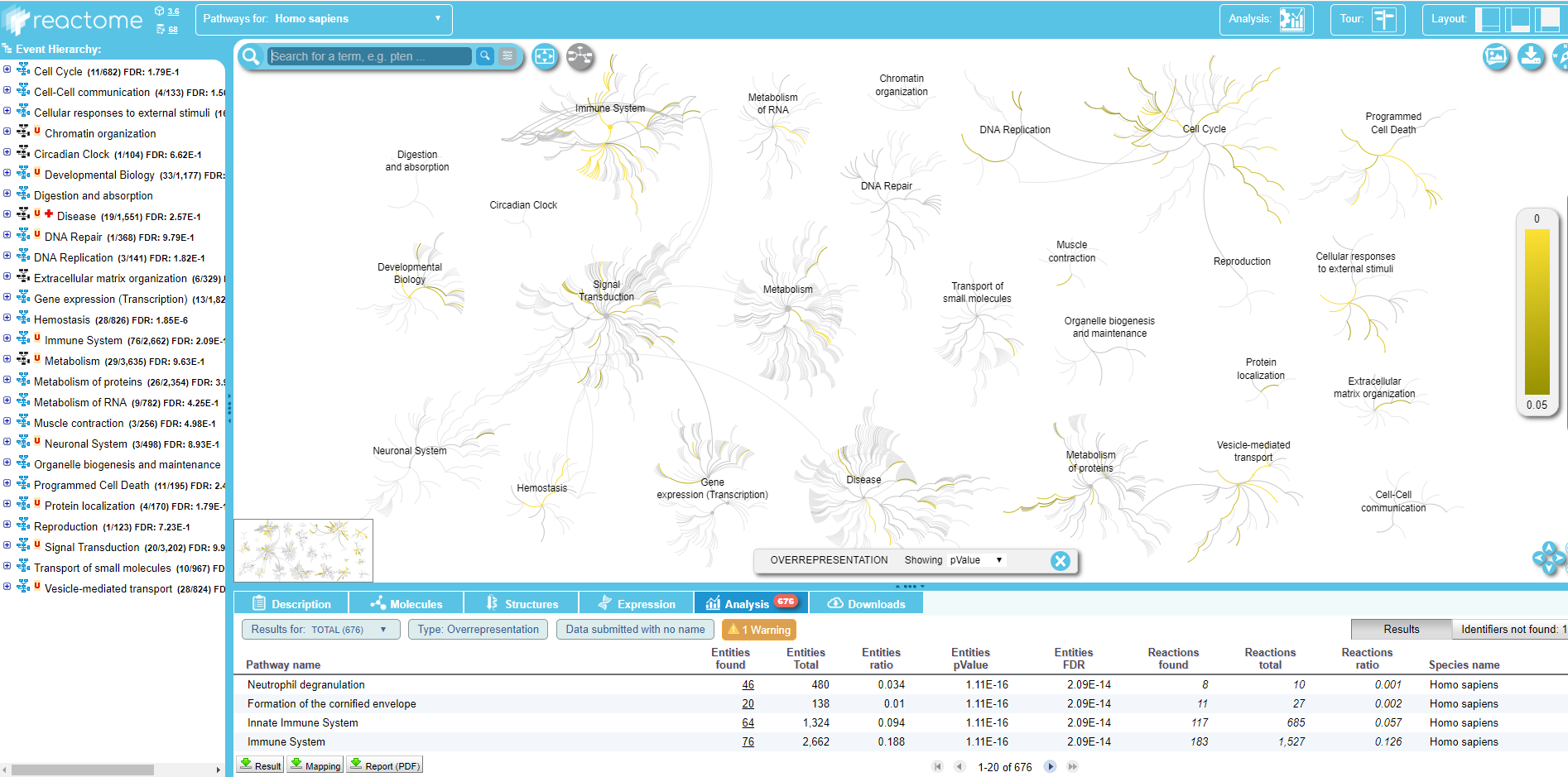Here you can explore the Reactome map of your IDs to see the context of your biological pathways.

Comparison with other proteomic datasets from previous studies

Hands-on: Lists comparison with Venn diagramm tool

1. Venn diagram tool with the following parameters:
   • param-repeat “Insert List to compare”
     • “Enter your list”: Input file containing your list
     • param-file “Select your file”: kept_lines (output of Filter by keywords and/or numerical value tool)
     • “Enter the name of this list”: Lacombe et al
   • param-repeat “Insert List to compare”
     • “Enter your list”: Input file containing your list
     • param-file “Select your file”: output (Input dataset)
     • “Enter the name of this list”: Bredberg et al
   • param-repeat “Insert List to compare”
     • “Enter your list”: Input file containing your list
     • param-file “Select your file”: output (Input dataset)
     • “Enter the name of this list”: Mucilli et al

Comment: Output

The Venn diagram shows the number of proteins specific and in common between the 3 lists. .

Conclusion

ProteoRE offers a panel of tools to annotate a protein list. We showed that it is possible to make ID conversion, perform tissu-expression annotation, but also Gene Ontology analysis as well as Reactome interogation. This allows the user to go deeper in the analysis of proteomics analyses results.

You've Finished the Tutorial

Please also consider filling out the Feedback Form as well!

Key points

• The Human Protein Atlas is a valuable resource for annotation and exploration of protein data

• Conversion between different gene identifiers is sometimes required

• The Reactome pathway database can be used to browse biological pathways

Frequently Asked Questions

Useful literature

Further information, including links to documentation and original publications, regarding the tools, analysis techniques and the interpretation of results described in this tutorial can be found here.

References

1. Uhlén, M., E. Björling, C. Agaton, C. A.-K. Szigyarto, B. Amini et al., 2005 A Human Protein Atlas for Normal and Cancer Tissues Based on Antibody Proteomics. Molecular & Cellular Proteomics 4: 1920–1932. 10.1074/mcp.m500279-mcp200
2. Bredberg, A., J. Gobom, A.-C. Almstrand, P. Larsson, K. Blennow et al., 2011 Exhaled Endogenous Particles Contain Lung Proteins. Clinical Chemistry 58: 431–440. 10.1373/clinchem.2011.169235
3. Croft, D., A. F. Mundo, R. Haw, M. Milacic, J. Weiser et al., 2013 The Reactome pathway knowledgebase. Nucleic acids research 42: D472–D477.
4. Muccilli, V., R. Saletti, V. Cunsolo, J. Ho, E. Gili et al., 2015 Protein profile of exhaled breath condensate determined by high resolution mass spectrometry. Journal of pharmaceutical and biomedical analysis 105: 134–149.
5. Lacombe, M., C. Marie-Desvergne, F. Combes, A. Kraut, C. Bruley et al., 2018 Proteomic characterization of human exhaled breath condensate. Journal of Breath Research 12: 021001. 10.1088/1752-7163/aa9e71

Feedback

Did you use this material as an instructor? Feel free to give us feedback on how it went.
Did you use this material as a learner or student? Click the form below to leave feedback.

Citing this Tutorial

1. Valentin Loux, Florence Combes, David Christiany, Yves Vandenbrouck, Annotating a protein list identified by LC-MS/MS experiments (Galaxy Training Materials). https://training.galaxyproject.org/training-material/topics/proteomics/tutorials/proteome_annotation/tutorial.html Online; accessed TODAY
2. Hiltemann, Saskia, Rasche, Helena et al., 2023 Galaxy Training: A Powerful Framework for Teaching! PLOS Computational Biology 10.1371/journal.pcbi.1010752
3. Batut et al., 2018 Community-Driven Data Analysis Training for Biology Cell Systems 10.1016/j.cels.2018.05.012

BibTeX

@misc{proteomics-proteome_annotation,
author = "Valentin Loux and Florence Combes and David Christiany and Yves Vandenbrouck",
	title = "Annotating a protein list identified by LC-MS/MS experiments (Galaxy Training Materials)",
	year = "",
	month = "",
	day = "",
	url = "\url{https://training.galaxyproject.org/training-material/topics/proteomics/tutorials/proteome_annotation/tutorial.html}",
	note = "[Online; accessed TODAY]"
}
@article{Hiltemann_2023,
	doi = {10.1371/journal.pcbi.1010752},
	url = {https://doi.org/10.1371%2Fjournal.pcbi.1010752},
	year = 2023,
	month = {jan},
	publisher = {Public Library of Science ({PLoS})},
	volume = {19},
	number = {1},
	pages = {e1010752},
	author = {Saskia Hiltemann and Helena Rasche and Simon Gladman and Hans-Rudolf Hotz and Delphine Larivi{\`{e}}re and Daniel Blankenberg and Pratik D. Jagtap and Thomas Wollmann and Anthony Bretaudeau and Nadia Gou{\'{e}} and Timothy J. Griffin and Coline Royaux and Yvan Le Bras and Subina Mehta and Anna Syme and Frederik Coppens and Bert Droesbeke and Nicola Soranzo and Wendi Bacon and Fotis Psomopoulos and Crist{\'{o}}bal Gallardo-Alba and John Davis and Melanie Christine Föll and Matthias Fahrner and Maria A. Doyle and Beatriz Serrano-Solano and Anne Claire Fouilloux and Peter van Heusden and Wolfgang Maier and Dave Clements and Florian Heyl and Björn Grüning and B{\'{e}}r{\'{e}}nice Batut and},
	editor = {Francis Ouellette},
	title = {Galaxy Training: A powerful framework for teaching!},
	journal = {PLoS Comput Biol}
}

                   

Galaxy Administrators: Install the missing tools

You can use Ephemeris's shed-tools install command to install the tools used in this tutorial.

shed-tools install [-g GALAXY] [-a API_KEY] -t <(curl https://training.galaxyproject.org/training-material/api/topics/proteomics/tutorials/proteome_annotation/tutorial.json | jq .admin_install_yaml -r)

Alternatively you can copy and paste the following YAML

---
install_tool_dependencies: true
install_repository_dependencies: true
install_resolver_dependencies: true
tools:
- name: proteore_clusterprofiler
  owner: proteore
  revisions: 2f67202ffdb3
  tool_panel_section_label: Proteomics
  tool_shed_url: https://toolshed.g2.bx.psu.edu/
- name: proteore_expression_rnaseq_abbased
  owner: proteore
  revisions: dbeabf9bf091
  tool_panel_section_label: Proteomics
  tool_shed_url: https://toolshed.g2.bx.psu.edu/
- name: proteore_filter_keywords_values
  owner: proteore
  revisions: b4641c0f8a82
  tool_panel_section_label: Proteomics
  tool_shed_url: https://toolshed.g2.bx.psu.edu/
- name: proteore_id_converter
  owner: proteore
  revisions: 1e45ea50f145
  tool_panel_section_label: Proteomics
  tool_shed_url: https://toolshed.g2.bx.psu.edu/
- name: proteore_reactome
  owner: proteore
  revisions: 9cc475dcd0f2
  tool_panel_section_label: Proteomics
  tool_shed_url: https://toolshed.g2.bx.psu.edu/
- name: proteore_reactome
  owner: proteore
  revisions: 6c95f1b88627
  tool_panel_section_label: Proteomics
  tool_shed_url: https://toolshed.g2.bx.psu.edu/
- name: proteore_tissue_specific_expression_data
  owner: proteore
  revisions: 3e65e0249976
  tool_panel_section_label: Proteomics
  tool_shed_url: https://toolshed.g2.bx.psu.edu/
- name: proteore_venn_diagram
  owner: proteore
  revisions: 98b7912a9ceb
  tool_panel_section_label: Proteomics
  tool_shed_url: https://toolshed.g2.bx.psu.edu/

Feedback

5 stars	6
4 stars	1
2 stars	1

March 2022

• 5 stars: Liked: Basics explained and accessible, which can be improved to acquire advanced skills and knowledge. thanks. Disliked: n/a

September 2021

• 5 stars: Liked: Really clear

April 2021

• 5 stars: Liked: really detailed and clear! Disliked: some tools have different names (e.g. it's now 'Pathway enrichment analysis [Reactome]' instead of 'Query pathway database [Reactome]', I think; in other words I couldn't find 'Query pathway database [Reactome]' so I improvised with 'Pathway enrichment analysis [Reactome]'). Also it would be good to include some tools to analise data other than these 3 species.

November 2020

• 2 stars: Disliked: I couldn't get past the "filter" part of this exercise because it did not explicitly state what filter tool to use. Filter using what? Again, many of your modules are helpful, but just as many need a biologist that is not a bioinformatics expert to help you understand where your directions are not clear. This module seems to have been edited by people that know bioinformatics, so all the stuff that's obvious to them isn't caught.