Molecular dynamics simulations return highly complex data. The Cartesian positions of each atom of the system (thousands or even millions) are recorded at every time step of the trajectory; this may again be thousands to millions of steps in length. Therefore, some kind of further analysis is needed to extract useful information from the data.

In this tutorial, we illustrate some of the analytical tools able to investigate conformational changes by analysis of a typical short protein simulation, such as for CBH1.

There are other analysis tools available; you are encouraged to try these out too.

Agenda

In this tutorial, we will cover:

1. Get data
2. Analysis with BIO3D
   1. RMSD
   2. RMSF
   3. PCA
   4. Workflow vs. individual tools
3. Further analysis
4. Conclusion

Get data

The data required can be generated by completing the NAMD simulation tutorial. Access it from your history. Alternatively, download the data from the Zenodo link provided.

Hands-on: Upload cellulose simulation trajectory

1. Create a new history

   Tip: Creating a new history

   To create a new history simply click the new-history icon at the top of the history panel:

   

2. Import the files from Zenodo, or from your history, if you completed the previous NAMD simulation tutorial:

   https://zenodo.org/record/2537734/files/cbh1test.dcd
   https://zenodo.org/record/2537734/files/cbh1test.pdb
   

   Tip: Importing via links

   • Copy the link location

   • Click galaxy-upload Upload Data at the top of the tool panel

   • Select galaxy-wf-edit Paste/Fetch Data

   • Paste the link(s) into the text field

   • Press Start

   • Close the window

3. Rename the dcd file ‘CBH1 trajectory’ and rename the pdb file ‘CBH1 structure’

   Tip: Renaming a dataset

   • Click on the galaxy-pencil pencil icon for the dataset to edit its attributes
   • In the central panel, change the Name field
   • Click the Save button

Analysis with BIO3D

We’ll carry out some basic analysis by calculating RMSD, RMSF and PCA. The tools use the Bio3D package, developed by the Grant lab.

RMSD

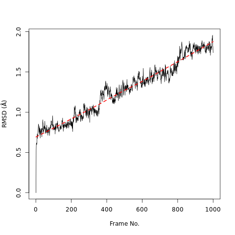
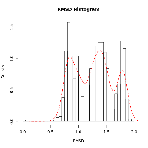
RMSD, or root-mean-square deviation, is a standard measure of structural distance between coordinates. It measures the average distance between a group of atoms (e.g. backbone atoms of a protein). If we calculate RMSD between two sets of atomic coordinates - for example, two time points from the trajectory - the value is a measure of how much the protein conformation has changed. Wikipedia provides more information.

Hands-on: Calculate RMSD

RMSD Analysis ( Galaxy version 2.3.4) with the following parameters:

• param-file “dcd trajectory input”: Trajectory file
• param-file “pdb input”: Structure file
• “Select domains”: Calpha (calculate RMSD only for the C-alpha domain of the protein)

Open image in new tab

Open image in new tab

Question

What do the features in the RMSD plot tell us?

Solution

The increase in the RMSD plot with time shows the protein steadily deviates from its original conformation.

The three peaks visible in the histogram suggests the presence of three main conformations which are accessed during the trajectory.

RMSF

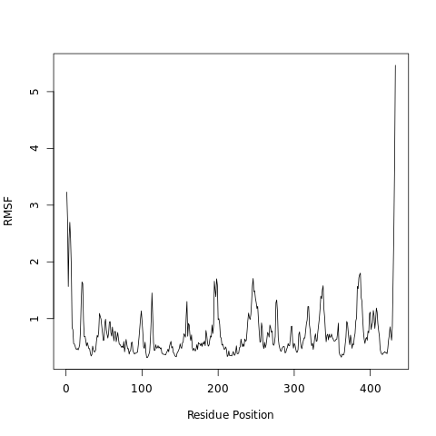
The root-mean-square fluctuation (RMSF) measures the average deviation of a particle (e.g. a protein residue) over time from a reference position (typically the time-averaged position of the particle). Thus, RMSF analyzes the portions of structure that are fluctuating from their mean structure the most (or least).

Hands-on: Calculate RMSF

1. RMSF Analysis ( Galaxy version 2.3.4) with the following parameters:
   • param-file “dcd trajectory input”: Trajectory file
   • param-file “pdb input”: Structure file
   • “Select domains”: Calpha (calculate RMSF only for the C-alpha domain of the protein)

Open image in new tab

Question

What can we learn from the features in the RMSF plot?

Solution

Higher RMSF values most likely are loop regions with more conformational flexibility, where the structure is not as well defined.

This allows a link with experimental spectroscopic techniques which detect the secondary structure of a protein.

PCA

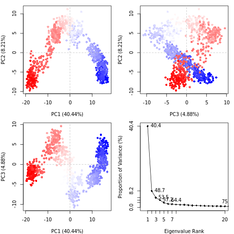
Principal component analysis (PCA) converts a set of correlated observations (movement of all atoms in protein) to a set of principal components which are linearly independent (or uncorrelated). Mathematically, it is a transformation of the data to a new coordinate system, in which the first coordinate represents the greatest variance, the second coordinate represents the second most variance, and so on.

You can read more about PCA on Wikipedia. In a nutshell, PCA takes a complex dataset with many variables and tries to distill the variables down to a few ‘principal components’ which still preserve most of the differences between the data.

In summary:

• The PCA tool tool will calculate and return a PCA to determine the relationship between statistically meaningful conformations (major global motions) sampled during the trajectory. THe tool returns several images of the PCA and the raw data in tab-separated format.
• The PCA visualization tool tool will carry out PCA and return a trajectory of the selected principle component. This trajectory is useful for visualisation and further investigating the interesting modes and changes that occur within a selected principle component.

Hands-on: Calculate PCA

1. PCA ( Galaxy version 2.3.4) with the following parameters:
   • param-file “dcd trajectory input”: Trajectory file
   • param-file “pdb input”: Structure file
   • “Use singular value decomposition (SVD) instead of default eigenvalue decomposition ?”: No
   • “Select domains”: Calpha
2. PCA visualization ( Galaxy version 2.3.4) with the following parameters:
   • param-file “dcd trajectory input”: Trajectory file
   • param-file “pdb input”: Structure file
   • “Use singular value decomposition (SVD) instead of default eigenvalue decomposition ?”: No
   • “Select domains”: Calpha
   • “Principal component id”: 1

PCA visualisation: This tool can generate small trajectories of the first three principal components. The .pdb of the .nc files can be visualized using a visualization software such as VMD.

Open image in new tab

Question

What do the features in the RMSD plot tell us? Do the principal coordinates have a meaning?

Solution

Here, PCA shows the statistically meaningful conformations in the CBH1 trajectory. The principal motions within the trajectory and the vital motions needed for conformational changes can be identified. Two distinct groupings along the PC1 plane, indicating a non-periodic conformational change, are identified. The groupings along the PC2 and PC3 planes do not completely cluster separately, implying that these global motions are periodic. The PC1 is linked to an active site motion that limits the motion to a key glycosidic bond.

Workflow vs. individual tools

You can choose to use the tools one by one as described above, or alternatively combine into a single analysis using the workflow provided.

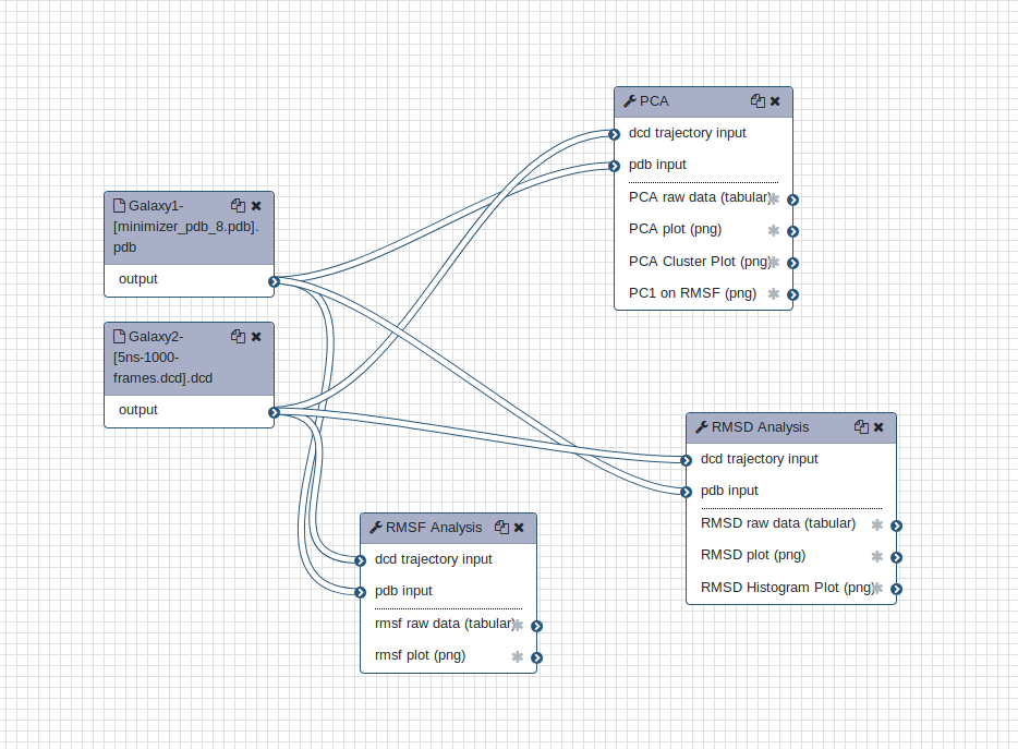Open image in new tab

Hands-on: Upload a workflow

1. Click on ‘Workflow’ in the toolbar at the top of the main Galaxy page. In the upper right corner of the central pane, click the ‘Upload or import workflow’ icon.

2. Enter the ‘Archived workflow URL’ and click ‘Import workflow’.

   https://raw.githubusercontent.com/galaxyproject/training-material/master/topics/computational-chemistry/tutorials/analysis-md-simulations/workflows/main_workflow.ga
   

Further analysis

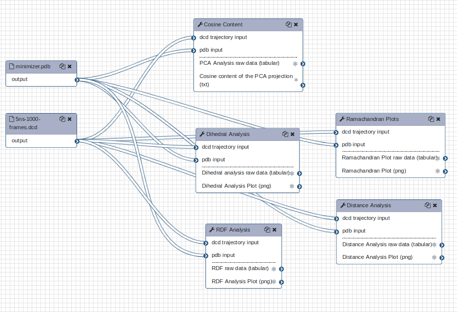
Further analyses are available; try out the MDAnalysis workflow, which includes a Ramachandran plot and various timeseries.

Open image in new tab

Conclusion

You've Finished the Tutorial

Please also consider filling out the Feedback Form as well!

Key points

• Multiple analyses including timeseries, RMSD, PCA are available

• Analysis tools allow a further chemical understanding of the system

Frequently Asked Questions

Useful literature

Further information, including links to documentation and original publications, regarding the tools, analysis techniques and the interpretation of results described in this tutorial can be found here.

Feedback

Did you use this material as an instructor? Feel free to give us feedback on how it went.
Did you use this material as a learner or student? Click the form below to leave feedback.

Citing this Tutorial

1. Christopher Barnett, Tharindu Senapathi, Simon Bray, Nadia Goué, Analysis of molecular dynamics simulations (Galaxy Training Materials). https://training.galaxyproject.org/training-material/topics/computational-chemistry/tutorials/analysis-md-simulations/tutorial.html Online; accessed TODAY
2. Hiltemann, Saskia, Rasche, Helena et al., 2023 Galaxy Training: A Powerful Framework for Teaching! PLOS Computational Biology 10.1371/journal.pcbi.1010752
3. Batut et al., 2018 Community-Driven Data Analysis Training for Biology Cell Systems 10.1016/j.cels.2018.05.012

BibTeX

@misc{computational-chemistry-analysis-md-simulations,
author = "Christopher Barnett and Tharindu Senapathi and Simon Bray and Nadia Goué",
	title = "Analysis of molecular dynamics simulations (Galaxy Training Materials)",
	year = "",
	month = "",
	day = "",
	url = "\url{https://training.galaxyproject.org/training-material/topics/computational-chemistry/tutorials/analysis-md-simulations/tutorial.html}",
	note = "[Online; accessed TODAY]"
}
@article{Hiltemann_2023,
	doi = {10.1371/journal.pcbi.1010752},
	url = {https://doi.org/10.1371%2Fjournal.pcbi.1010752},
	year = 2023,
	month = {jan},
	publisher = {Public Library of Science ({PLoS})},
	volume = {19},
	number = {1},
	pages = {e1010752},
	author = {Saskia Hiltemann and Helena Rasche and Simon Gladman and Hans-Rudolf Hotz and Delphine Larivi{\`{e}}re and Daniel Blankenberg and Pratik D. Jagtap and Thomas Wollmann and Anthony Bretaudeau and Nadia Gou{\'{e}} and Timothy J. Griffin and Coline Royaux and Yvan Le Bras and Subina Mehta and Anna Syme and Frederik Coppens and Bert Droesbeke and Nicola Soranzo and Wendi Bacon and Fotis Psomopoulos and Crist{\'{o}}bal Gallardo-Alba and John Davis and Melanie Christine Föll and Matthias Fahrner and Maria A. Doyle and Beatriz Serrano-Solano and Anne Claire Fouilloux and Peter van Heusden and Wolfgang Maier and Dave Clements and Florian Heyl and Björn Grüning and B{\'{e}}r{\'{e}}nice Batut and},
	editor = {Francis Ouellette},
	title = {Galaxy Training: A powerful framework for teaching!},
	journal = {PLoS Comput Biol}
}

                   

Go Further

Do you want to extend your knowledge? Follow one of our recommended follow-up trainings:

• tutorial Hands-on: Analysis of molecular dynamics simulations

Galaxy Administrators: Install the missing tools

You can use Ephemeris's shed-tools install command to install the tools used in this tutorial.

shed-tools install [-g GALAXY] [-a API_KEY] -t <(curl https://training.galaxyproject.org/training-material/api/topics/computational-chemistry/tutorials/analysis-md-simulations/tutorial.json | jq .admin_install_yaml -r)

Alternatively you can copy and paste the following YAML

---
install_tool_dependencies: true
install_repository_dependencies: true
install_resolver_dependencies: true
tools:
- name: bio3d_pca
  owner: chemteam
  revisions: 994c509873db
  tool_panel_section_label: ChemicalToolBox
  tool_shed_url: https://toolshed.g2.bx.psu.edu/
- name: bio3d_pca
  owner: chemteam
  revisions: 24867ab16f36
  tool_panel_section_label: ChemicalToolBox
  tool_shed_url: https://toolshed.g2.bx.psu.edu/
- name: bio3d_rmsd
  owner: chemteam
  revisions: f871c9a8cb7c
  tool_panel_section_label: ChemicalToolBox
  tool_shed_url: https://toolshed.g2.bx.psu.edu/
- name: bio3d_rmsd
  owner: chemteam
  revisions: 77e28e1da9f4
  tool_panel_section_label: ChemicalToolBox
  tool_shed_url: https://toolshed.g2.bx.psu.edu/
- name: bio3d_rmsf
  owner: chemteam
  revisions: 4354d92dc1aa
  tool_panel_section_label: ChemicalToolBox
  tool_shed_url: https://toolshed.g2.bx.psu.edu/
- name: bio3d_rmsf
  owner: chemteam
  revisions: 6bcb804a54c3
  tool_panel_section_label: ChemicalToolBox
  tool_shed_url: https://toolshed.g2.bx.psu.edu/
- name: mdanalysis_cosine_analysis
  owner: chemteam
  revisions: ebeb72aa39a8
  tool_panel_section_label: ChemicalToolBox
  tool_shed_url: https://toolshed.g2.bx.psu.edu/
- name: mdanalysis_dihedral
  owner: chemteam
  revisions: 554f60da9c8f
  tool_panel_section_label: ChemicalToolBox
  tool_shed_url: https://toolshed.g2.bx.psu.edu/
- name: mdanalysis_distance
  owner: chemteam
  revisions: 489b25966bb9
  tool_panel_section_label: ChemicalToolBox
  tool_shed_url: https://toolshed.g2.bx.psu.edu/
- name: mdanalysis_ramachandran_plot
  owner: chemteam
  revisions: d710c7f00ae6
  tool_panel_section_label: ChemicalToolBox
  tool_shed_url: https://toolshed.g2.bx.psu.edu/
- name: mdanalysis_rdf
  owner: chemteam
  revisions: 49dac57d004a
  tool_panel_section_label: ChemicalToolBox
  tool_shed_url: https://toolshed.g2.bx.psu.edu/

Feedback

5 stars	2
4 stars	3
1 stars	1

October 2023

• 5 stars: Liked: Extremely easy to follow and I was so impressed that it all works as described. Good maintenance :) Disliked: I had the mental model of a Jupyter Notebook coming in, so I was trying to figure out how to open the tutorial in my usegalaxy.org account view.

January 2023

• 4 stars: Liked: The interpretation of RMSD, RMSF, and PCA plots.

February 2022

• 4 stars: Disliked: The further analysis links seems to be broken/unavailable: https://github.com/galaxyproject/training-material/tree/main/topics/computational-chemistry/tutorials/analysis-md-simulations/workflows/advanced_workflow.ga

October 2021

• 1 stars: Liked: yes Disliked: yes

May 2020

• 4 stars: Disliked: Analysis of Rg, Hydrogen bonds can also be explained