De Bruijn Graph Assembly
| Author(s) |
|
| Editor(s) |
|
| Reviewers |
|
OverviewQuestions:
Objectives:
What are the factors that affect genome assembly?
How does Genome assembly work?
Requirements:
Perform an optimised Velvet assembly with the Velvet Optimiser
Compare this assembly with those we did in the basic tutorial
Perform an assembly using the SPAdes assembler.
Time estimation: 2 hoursLevel: Introductory IntroductorySupporting Materials:Published: May 24, 2017Last modification: Jan 7, 2026License: Tutorial Content is licensed under Creative Commons Attribution 4.0 International License. The GTN Framework is licensed under MITpurl PURL: https://gxy.io/GTN:T00031rating Rating: 2.9 (0 recent ratings, 9 all time)version Revision: 26
Optimised de Bruijn Graph assemblies using the Velvet Optimiser and SPAdes
In this activity, we will perform de novo assemblies of a short read set using the Velvet Optimiser and the SPAdes assemblers. We are using the Velvet Optimiser for illustrative purposes. For real assembly work, a more suitable assembler should be chosen - such as SPAdes.
The Velvet Optimiser is a script written by
Simon Gladman
to optimise the k-mer size and coverage cutoff parameters for Velvet. More information can be found in its repository.
SPAdes is a de novo genome assembler written by Pavel Pevzner’s group in St. Petersburg. More details on it can be found on Spades’ website>
AgendaIn this tutorial, we will deal with:
Get the data
We will be using the same data that we used in the introductory tutorial, so if you have already completed that and have the data, skip this section.
Hands On: Getting the data
Create and name a new history for this tutorial.
To create a new history simply click the new-history icon at the top of the history panel:
Import the sequence read raw data (*.fastq) from Zenodo
https://zenodo.org/record/582600/files/mutant_R1.fastq
https://zenodo.org/record/582600/files/mutant_R2.fastq
- Copy the link location
Click galaxy-upload Upload at the top of the activity panel
- Select galaxy-wf-edit Paste/Fetch Data
Paste the link(s) into the text field
Press Start
- Close the window
- Rename the files galaxy-pencil
- The name of the files are the full URL, let’s make the names a little clearer
- Change the names to just the last part,
Mutant_R1.fastq,Mutant_R2.fastq, respectively
- Click on the galaxy-pencil pencil icon for the dataset to edit its attributes
- In the central panel, change the Name field
- Click the Save button
Question
- What are four key features of a FASTQ file?
- What is the main difference between a FASTQ and a FASTA file?
Create a paired collection named
Paired Reads
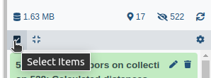
- Click on galaxy-selector Select Items at the top of the history panel
- Check all the datasets in your history you would like to include
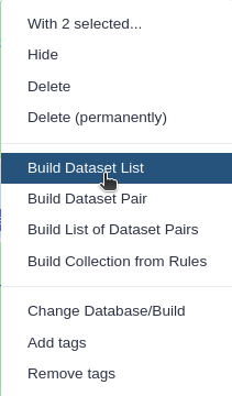
Click n of N selected and choose Advanced Build List
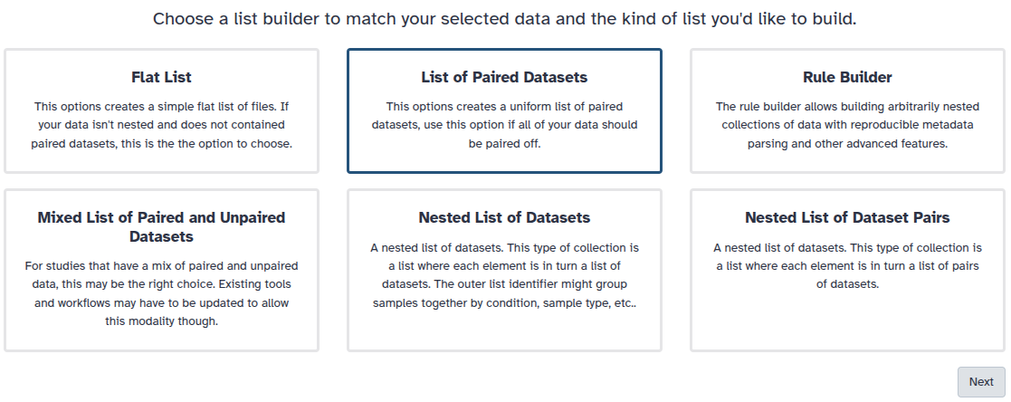
You are in the collection building wizard. Choose List of Paired Datasets and click ‘Next’ button at the right bottom corner.
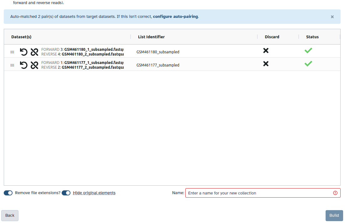
Check and configure auto-pairing. Commonly matepairs have suffix
_1and_2or_R1and_R2. Click on ‘Next’ at the bottom.
- Edit the List Identifier as required.
- Enter a name for your collection
- Click Build to build your collection
- Click on the checkmark icon at the top of your history again
- We will need to use both the individual datasets (
Mutant_R1.fastqandMutant_R2.fastq) and the paired end collection (Paired Reads), so toggle off theHide original elementsoption when creating the collection.- Alternatively, you can un-hide the datasets by selecting the galaxy-show-hidden icon on the hidden dataset in your history.
If your history contains hidden datasets you will see galaxy-show-hidden “Include hidden” button directly above the dataset display.
To un-hide datasets:
- Type
visible:hiddenin the search box- Select datasets you want to un-hide
- Click the dropdown that would appear at the top of the history;
- Select “Unhide” option.
Alternatively, you can:
- click galaxy-show-hidden “Include hidden” button directly above dataset display. This will cause hidden datasets to appear in history along with normal (un-hidden) datasets;
- hidden datasets are distinguished by having galaxy-show-hidden within dataset box. Clicking on this icon will un-hide a given dataset;


Assembly with the Velvet Optimiser
We will perform an assembly with the Velvet Optimiser, which automatically runs and optimises the output of the Velvet assembler (Zerbino and Birney 2008). It will automatically choose a suitable value for the k-mer size (k). It will then go on to optimise the coverage cutoff (cov_cutoff) which corrects for read errors. It will use the “n50” metric for optimising the k-mer size and the “total number of bases in contigs” for optimising the coverage cutoff.
Hands On: Assemble with the Velvet Optimiser
- Velvet Optimiser ( Galaxy version 2.2.6): Optimise your assembly with the following parameters:
- “Start k-mer size”:
45- “End k-mer size”:
73- “Input Files”:
1: Input Files
- “Input file type”:
Fastq- “Single or paired end reads”:
Paired- param-file “Select first set of reads”:
mutant_R1.fastq- param-file “Select second set of reads”:
mutant_R2.fastq
Your history will now contain a number of new files:
- Velvet optimiser contigs
- A fasta file of the final assembled contigs
- Velvet optimiser contig stats
- A table of the lengths (in k-mer length) and coverages (k-mer coverages) for the final contigs.
Have a look at each file.
Hands On: Get contig statistics for Velvet Optimiser contigs
- Fasta Statistics ( Galaxy version 1.0.1): Produce a summary of the velvet optimiser contigs:
- param-file “fasta or multifasta file”: Select your velvet optimiser contigs file
View the output
QuestionCompare the output we got here with the output of the simple assemblies obtained in the introductory tutorial.
- What are the main differences between them?
- Which has a higher “n50”? What does this mean?
Tables of results from (a) Simple assembly and (b) optimised assembly.
(a) 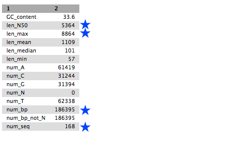
(b) 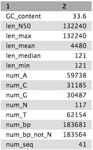
- Heuristic Resolution of Repeats and Scaffolding in the Velvet Short-Read de Novo Assembler (Zerbino et al. 2009)
Visualisation of the Assembly
Now that we’ve assembled the genomes, let’s visualise this assembly using Bandage (Wick et al. 2015). This tool will let us better understand how the assembly graph really looks, and can give us a feeling for if the genome was well assembled or not.
Currently VelvetOptimiser does not include the LastGraph output, so we will manually run velveth and velvetg with the optimised parameters.
Hands On: Manually running velvetg/h
Locate the output called “VelvetOptimiser: Contigs” in your history
Click the dataset-info information icon
Check the tool
stderrin the information page for the optimised k-mer value
QuestionWhat was the optimal k-mer value? (referred to as “hash” in the stderr log)
55
With this information in hand, let’s run velvet:
Hands On: Manually running velvetg/h
- velveth ( Galaxy version 1.2.10.3): Prepare a dataset for the Velvet
velvetgAssembler
- “Hash length”:
55- “Input Files”:
+ Insert Input Files1: Input Files
- “Choose the input type”:
separate paired reads- “read type”:
shortPaired reads- “Dataset”:
mutant_R1.fastq(forward reads)- “Dataset”:
mutant_R2.fastq(reverse reads)- velvetg ( Galaxy version 1.2.10.2): Velvet sequence assembler for very short reads
- “Velvet dataset”: output from velveth tool
- “Coverage cutoff”:
Specify Cutoff Value
- “Remove nodes with coverage below”:
1.44- “Additional outputs”:
Generate velvet LastGraph file- “Using Paired Reads”:
Yes
The LastGraph contains a detailed representation of the De Bruijn graph, which can give us an idea how velvet has assembled the genome and potentially resolved any conflicts.
Hands On: Bandage
- Bandage Image ( Galaxy version 2022.09+galaxy4): visualize de novo assembly graphs
- “Graphical Fragment Assembly”: The “LastGraph” output of velvetg tool
- “Produce jpg, png or svg file?”:
.png- Execute
- View the output file
And now you should be able to see the graph that velvet produced:

Interpreting Bandage Graphs
k-mer size has a significant effect on the assembly. You can play around with various k-mers to see this effect in practice.
| k-mer | graph |
|---|---|
| 21 |  |
| 33 |  |
| 53 |  |
| 77 |  |
The next thing to be aware of is that there can be multiple valid interpretations of a graph, all equally valid in absence of other data. The following is taken verbatim from Bandage’s wiki:
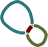
For a simple case, imagine a bacterial genome that contains a single repeated element in two separate places in the chromosome:
A researcher (who does not yet know the structure of the genome) sequences it, and the resulting 100 bp reads are assembled with a de novo assembler:
Because the repeated element is longer than the sequencing reads, the assembler was not able to reproduce the original genome as a single contig. Rather, three contigs are produced: one for the repeated sequence (even though it occurs twice) and one for each sequence between the repeated elements.
Given only the contigs, the relationship between these sequences is not clear. However, the assembly graph contains additional information which is made apparent in Bandage:
There are two principal underlying sequences compatible with this graph: two separate circular sequences that share a region in common, or a single larger circular sequence with an element that occurs twice:
Additional knowledge, such as information on the approximate size of the bacterial chromosome, can help the researcher to rule out the first alternative. In this way, Bandage has assisted in turning a fragmented assembly of three contigs into a completed genome of one sequence.


Assemble with SPAdes
We will now perform an assembly with the much more modern SPAdes assembler (Bankevich et al. 2012). It goes through a similar process to Velvet in the fact that it uses and simplifies de Bruijn graphs but it uses multiple values for k-mer size and combines the resultant graphs. This combination produces very good assemblies. When using SPAdes it is typical to choose at least 3 k-mer sizes. One low, one medium and one high. We will use 33, 55 and 91.
Hands On: Assemble with SPAdes
- SPAdes ( Galaxy version 4.2.0+galaxy0): Assemble the reads:
- “Operation mode”:
Only assembler (--only_assembler)- “Single-end or paired-end short-reads”:
Paired-end: list of dataset pairs
- “FASTA/FASTQ file(s): collection”:
Paired Reads- “Set coverage cutoff option”:
auto- “Select k-mer detection option”:
User specific
- “K-mer size values”:
33,55,91[note: no spaces!]- “Select optional output file(s)”:
Assembly graph,Assembly graph with scaffold,Contigs,Scaffolds,Log
You will now have 5 new files in your history:
- two Fasta files, one for contigs and one for scaffolds
- two statistics files, one for contigs and one for scaffolds
- the SPAdes log file.
Examine each file, especially the stats files.
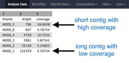
Question
- Why would one of the contigs have much higher coverage than the others?
- What could this represent?
Hands On: Visualize assembly with Bandage
- Bandage Image ( Galaxy version 2022.09+galaxy4) with the following parameters:
- “Graphical Fragment Assembly”:
assembly graph with scaffoldsoutput from SPAdes tool- “Produce jpg, png or svg file?”:
.png- Examine the output image galaxy-eye
The visualized assembly should look something like this:

QuestionWhich assembly looks better to you? Why?
Hands On: Get contig statistics for SPAdes contigs
- Fasta Statistics ( Galaxy version 1.0.1): Produce a summary of the SPAdes contigs:
- param-file “fasta or multifasta file”: Select your velvet optimiser contigs file
Look at the output file.
QuestionCompare the output we got here with the output of the simple assemblies obtained in the introductory tutorial.
- What are the main differences between them?
- Did SPAdes produce a better assembly than the Velvet Optimiser?
You've Finished the Tutorial
Key points
We learned about how the choice of k-mer size will affect assembly outcomes
We learned about the strategies that assemblers use to make reference genomes
We performed a number of assemblies with Velvet and SPAdes.
You should use SPAdes or another more modern assembler than Velvet for actual assemblies now.
Frequently Asked Questions
Have questions about this tutorial? Have a look at the available FAQ pages and support channelsReferences
- Zerbino, D. R., and E. Birney, 2008 Velvet: Algorithms for de novo short read assembly using de Bruijn graphs. Genome Research 18: 821–829. 10.1101/gr.074492.107
- Zerbino, D. R., G. K. McEwen, E. H. Margulies, and E. Birney, 2009 Pebble and Rock Band: Heuristic Resolution of Repeats and Scaffolding in the Velvet Short-Read de Novo Assembler (S. L. Salzberg, Ed.). PLoS ONE 4: e8407. 10.1371/journal.pone.0008407
- Bankevich, A., S. Nurk, D. Antipov, A. A. Gurevich, M. Dvorkin et al., 2012 SPAdes: A New Genome Assembly Algorithm and Its Applications to Single-Cell Sequencing. Journal of Computational Biology 19: 455–477. 10.1089/cmb.2012.0021
- Wick, R. R., M. B. Schultz, J. Zobel, and K. E. Holt, 2015 Bandage: interactive visualization of \lessi\greaterde novo\less/i\greater genome assemblies. Bioinformatics 31: 3350–3352. 10.1093/bioinformatics/btv383
Feedback
Did you use this material as an instructor? Feel free to give us feedback on how it went.
Did you use this material as a learner or student? Click the form below to leave feedback.

Citing this Tutorial
- Simon Gladman, Helena Rasche, Saskia Hiltemann, De Bruijn Graph Assembly (Galaxy Training Materials). https://training.galaxyproject.org/training-material/topics/assembly/tutorials/debruijn-graph-assembly/tutorial.html Online; accessed TODAY
- Hiltemann, Saskia, Rasche, Helena et al., 2023 Galaxy Training: A Powerful Framework for Teaching! PLOS Computational Biology 10.1371/journal.pcbi.1010752
- Batut et al., 2018 Community-Driven Data Analysis Training for Biology Cell Systems 10.1016/j.cels.2018.05.012
@misc{assembly-debruijn-graph-assembly,
author = "Simon Gladman and Helena Rasche and Saskia Hiltemann",
	title = "De Bruijn Graph Assembly (Galaxy Training Materials)",
	year = "",
	month = "",
	day = "",
	url = "\url{https://training.galaxyproject.org/training-material/topics/assembly/tutorials/debruijn-graph-assembly/tutorial.html}",
	note = "[Online; accessed TODAY]"
}
@article{Hiltemann_2023,
	doi = {10.1371/journal.pcbi.1010752},
	url = {https://doi.org/10.1371%2Fjournal.pcbi.1010752},
	year = 2023,
	month = {jan},
	publisher = {Public Library of Science ({PLoS})},
	volume = {19},
	number = {1},
	pages = {e1010752},
	author = {Saskia Hiltemann and Helena Rasche and Simon Gladman and Hans-Rudolf Hotz and Delphine Larivi{\`{e}}re and Daniel Blankenberg and Pratik D. Jagtap and Thomas Wollmann and Anthony Bretaudeau and Nadia Gou{\'{e}} and Timothy J. Griffin and Coline Royaux and Yvan Le Bras and Subina Mehta and Anna Syme and Frederik Coppens and Bert Droesbeke and Nicola Soranzo and Wendi Bacon and Fotis Psomopoulos and Crist{\'{o}}bal Gallardo-Alba and John Davis and Melanie Christine Föll and Matthias Fahrner and Maria A. Doyle and Beatriz Serrano-Solano and Anne Claire Fouilloux and Peter van Heusden and Wolfgang Maier and Dave Clements and Florian Heyl and Björn Grüning and B{\'{e}}r{\'{e}}nice Batut and},
	editor = {Francis Ouellette},
	title = {Galaxy Training: A powerful framework for teaching!},
	journal = {PLoS Comput Biol}
}
Funding
These individuals or organisations provided funding support for the development of this resource
Congratulations on successfully completing this tutorial!
You can use Ephemeris's
shed-tools installcommand to install the tools used in this tutorial.shed-tools install [-g GALAXY] [-a API_KEY] -t <(curl https://training.galaxyproject.org/training-material/api/topics/assembly/tutorials/debruijn-graph-assembly/tutorial.json | jq .admin_install_yaml -r)Alternatively you can copy and paste the following YAML
---
install_tool_dependencies: true
install_repository_dependencies: true
install_resolver_dependencies: true
tools:
- name: velvet
  owner: devteam
  revisions: 920677cd220f
  tool_panel_section_label: Assembly
  tool_shed_url: https://toolshed.g2.bx.psu.edu/
- name: velvet
  owner: devteam
  revisions: 920677cd220f
  tool_panel_section_label: Assembly
  tool_shed_url: https://toolshed.g2.bx.psu.edu/
- name: bandage
  owner: iuc
  revisions: '067592b6b312'
  tool_panel_section_label: Graph/Display Data
  tool_shed_url: https://toolshed.g2.bx.psu.edu/
- name: bandage
  owner: iuc
  revisions: 86ec2f06de3c
  tool_panel_section_label: Graph/Display Data
  tool_shed_url: https://toolshed.g2.bx.psu.edu/
- name: fasta_stats
  owner: iuc
  revisions: 9c620a950d3a
  tool_panel_section_label: FASTA/FASTQ
  tool_shed_url: https://toolshed.g2.bx.psu.edu/
- name: spades
  owner: nml
  revisions: 822954de3f59
  tool_panel_section_label: Assembly
  tool_shed_url: https://toolshed.g2.bx.psu.edu/
- name: velvetoptimiser
  owner: simon-gladman
  revisions: 37d88f41c810
  tool_panel_section_label: Assembly
  tool_shed_url: https://toolshed.g2.bx.psu.edu/