Exome sequencing is a method that enables the selective sequencing of the exonic regions of a genome - that is the transcribed parts of the genome present in mature mRNA, including protein-coding sequences, but also untranslated regions (UTRs).

In humans, there are about 180,000 exons with a combined length of ~ 30 million base pairs (30 Mb). Thus, the exome represents only 1% of the human genome, but has been estimated to harbor up to 85% of all disease-causing variants (Choi et al., 2009).

Exome sequencing, thus, offers an affordable alternative to whole-genome sequencing in the diagnosis of genetic disease, while still covering far more potential disease-causing variant sites than genotyping arrays. This is of special relevance in the case of rare genetic diseases, for which the causative variants may occur at too low a frequency in the human population to be included on genotyping arrays.

Of note, a recent study focusing on the area of clinical pediatric neurology indicates that the costs of exome sequencing may actually not be higher even today than the costs of conventional genetic testing (Vissers et al., 2017).

Details: Exome sequencing vs whole-genome sequencing

In principle, the steps illustrated in this tutorial are suitable also for the analysis of whole-genome sequencing (WGS) data. At comparable mean coverage, however, WGS datasets will be much larger than exome sequencing ones and their analysis will take correspondingly more time.

The obvious benefit of WGS compared to exome-sequencing, of course, is that it will allow variant detection in even more regions of the genome. As a less apparent advantage, the more complete information of WGS data can make it easier to detect copy number variation (CNV) and structural variants such as translocations and inversions (although such detection will require more sophisticated analysis steps, which are not covered by this tutorial).

Very generally, one could argue that exome-sequencing captures most of the information that can be analyzed with standard bioinformatical tools today at reasonable costs. WGS, on the other hand, captures as much information as today’s sequencing technology can provide, and it may be possible to reanalyze such data with more powerful bioinformatical software in the future to exploit aspects of the information that were not amenable to analysis at the time of data acquisition.

The identification of causative variants underlying any particular genetic disease is, as we will see in this tutorial, not just dependent on the successful detection of variants in the genome of the patient, but also on variant comparison between the patient and selected relatives. Most often family trio data, consisting of the genome sequences of the patient and their parents, is used for this purpose. With multisample data like this it becomes possible to search for variants following any kind of Mendelian inheritance scheme compatible with the observed inheritance pattern of the disease, or to detect possibly causative de-novo mutations or loss-of-heterozygosity (LOH) events.

Details: Related tutorials

This tutorial focuses on the practical aspects of analyzing real-world patient data. If you are more interested in the theoretical aspects of variant calling, you may want to have a look at the related tutorial on Calling variants in diploid systems.

The tutorial on Somatic variant calling follows an analysis workflow that is rather similar to the one here, but tries to identify tumor variants by comparing a tumor sample to healthy tissue from the same patient. Together, the two tutorials are intended to get you started with genomics medicine using Galaxy.

Agenda

In this tutorial, we will cover:

1. Data Preparation
   1. Get data
2. Quality control
3. Read mapping
4. Mapped reads postprocessing
   1. Filtering on mapped reads properties
   2. Removing duplicate reads
5. Variant calling
   1. Generating FreeBayes calls
   2. Post-processing FreeBayes calls
6. Variant annotation and reporting
   1. Get data
   2. Variant annotation with functional genomic effects
   3. Generating a GEMINI database of variants for further annotation and efficient variant queries
   4. Candidate variant detection
7. Conclusion

Data Preparation

In this tutorial, we are going to analyze exome sequencing data from a family trio, in which the boy child is affected by the disease osteopetrosis, while both parents, who happen to be consanguineous, are unaffected. Our goal is to identify the genetic variation that is responsible for the disease.

Get data

tip This tutorial offers two alternative entry points allowing you to

• conduct a full analysis starting from original sequenced reads in fastq format or to
• start your analysis with premapped reads in bam format that are (almost) ready for variant calling.

While the full analysis is probably closer to how you would analyze your own data, the shortened analysis from premapped reads may suit your time frame better, and will avoid redundancy if you have previously worked through other tutorials demonstrating NGS quality control and read mapping, like the dedicated Quality control and Mapping tutorials.

The following hands-on section will guide you through obtaining the right data for either analysis.

Hands-on: Data upload

1. Create a new history for this tutorial and give it a meaningful name

   Tip: Creating a new history

   Click the new-history icon at the top of the history panel:

   

   Tip: Renaming a history

   1. Click on galaxy-pencil (Edit) next to the history name (which by default is “Unnamed history”)
   2. Type the new name
   3. Click on Save

   If you do not have the galaxy-pencil (Edit) next to the history name:

   1. Click on Unnamed history (or the current name of the history) (Click to rename history) at the top of your history panel
   2. Type the new name
   3. Press Enter

2. Obtain the raw sequencing data

   Comment: Starting from raw sequencing data

   In this and the following steps you will obtain the original unmapped sequencing data and prepare for a full analysis including the mapping of the sequenced reads.

   If you prefer to skip the mapping step and start the analysis from premapped data you should proceed directly to step 4 of this section.

   Import the original sequenced reads datasets of the family trio from Zenodo:

   https://zenodo.org/record/3243160/files/father_R1.fq.gz
   https://zenodo.org/record/3243160/files/father_R2.fq.gz
   https://zenodo.org/record/3243160/files/mother_R1.fq.gz
   https://zenodo.org/record/3243160/files/mother_R2.fq.gz
   https://zenodo.org/record/3243160/files/proband_R1.fq.gz
   https://zenodo.org/record/3243160/files/proband_R2.fq.gz
   

   Alternatively, the same files may be available on your Galaxy server through a shared data library (your instructor may tell you so), in which case you may prefer to import the data directly from there.

   Tip: Importing via links

   • Copy the link location

   • Click galaxy-upload Upload Data at the top of the tool panel

   • Select galaxy-wf-edit Paste/Fetch Data

   • Paste the link(s) into the text field

   • Change Type (set all): from “Auto-detect” to fastqsanger.gz

   • Press Start

   • Close the window

   Tip: Importing data from a data library

   As an alternative to uploading the data from a URL or your computer, the files may also have been made available from a shared data library:

   1. Go into Shared data (top panel) then Data libraries
   2. Navigate to the correct folder as indicated by your instructor.
      • On most Galaxies tutorial data will be provided in a folder named GTN - Material –> Topic Name -> Tutorial Name.
   3. Select the desired files
   4. Click on Add to History galaxy-dropdown near the top and select as Datasets from the dropdown menu

   5. In the pop-up window, choose

      • “Select history”: the history you want to import the data to (or create a new one)
   6. Click on Import

3. Check that the newly created datasets in your history have their datatypes assigned correctly to fastqsanger.gz, and fix any missing or wrong datatype assignment

   Tip: Changing the datatype

   • Click on the galaxy-pencil pencil icon for the dataset to edit its attributes
   • In the central panel, click galaxy-chart-select-data Datatypes tab on the top
   • In the galaxy-chart-select-data Assign Datatype, select fastqsanger.gz from “New type” dropdown
     • Tip: you can start typing the datatype into the field to filter the dropdown menu
   • Click the Save button

   trophy Congratulations for obtaining the datasets required for an analysis including reads mapping. You should now proceed with Step 7 below.

4. Obtain the premapped sequencing data

   Comment: Alternative entry point: Premapped data

   Skip this and the following two steps if you already obtained and prepared the original unmapped seuencing data and are planning to perform the mapping step yourself.

   Import the premapped reads datasets of the family trio from Zenodo:

   https://zenodo.org/record/3243160/files/mapped_reads_father.bam
   https://zenodo.org/record/3243160/files/mapped_reads_mother.bam
   https://zenodo.org/record/3243160/files/mapped_reads_proband.bam
   

   Alternatively, the same files may be available on your Galaxy server through a shared data library (your instructor may tell you so), in which case you may prefer to import the data directly from there.

   Tip: Importing via links

   • Copy the link location

   • Click galaxy-upload Upload Data at the top of the tool panel

   • Select galaxy-wf-edit Paste/Fetch Data

   • Paste the link(s) into the text field

   • Change Type (set all): from “Auto-detect” to bam

   • Press Start

   • Close the window

   Tip: Importing data from a data library

   As an alternative to uploading the data from a URL or your computer, the files may also have been made available from a shared data library:

   1. Go into Shared data (top panel) then Data libraries
   2. Navigate to the correct folder as indicated by your instructor.
      • On most Galaxies tutorial data will be provided in a folder named GTN - Material –> Topic Name -> Tutorial Name.
   3. Select the desired files
   4. Click on Add to History galaxy-dropdown near the top and select as Datasets from the dropdown menu

   5. In the pop-up window, choose

      • “Select history”: the history you want to import the data to (or create a new one)
   6. Click on Import

5. Check that the newly created datasets in your history have their datatypes assigned correctly to bam, and fix any missing or wrong datatype assignment

   Tip: Changing the datatype

   • Click on the galaxy-pencil pencil icon for the dataset to edit its attributes
   • In the central panel, click galaxy-chart-select-data Datatypes tab on the top
   • In the galaxy-chart-select-data Assign Datatype, select bam from “New type” dropdown
     • Tip: you can start typing the datatype into the field to filter the dropdown menu
   • Click the Save button

6. Specify the genome version that was used for mapping

   Change the database/build (dbkey) for each of your bam datasets to hg19.

   Tip: Changing database/build (dbkey)

   • Click the desired dataset’s name to expand it.

   • Click on the “?” next to database indicator:

     

   • In the central panel, change the Database/Build field
   • Select your desired database key from the dropdown list: Human Feb. 2009 (GRCh37/hg19) (hg19)
   • Click the Save button

   Details: Why specify genome versions

   When you are starting with sequencing data that has already been mapped to a particular genome version (human hg19 in this case), it is good practice to attach this information as metadata to the datasets.

   Doing so helps prevent accidental use of a different version of the reference genome in later steps like variant calling, which would typically lead to nonsensical results because of base position changes between the different versions.

   trophy Congratulations for obtaining the premapped sequencing datasets. Now, follow the remaining steps to set everything up for a successful analysis.

7. Rename the datasets

   For datasets that you upload via a link, Galaxy will pick the link address as the dataset name, which you will likely want to shorten to just the file names.

   Tip: Renaming a dataset

   • Click on the galaxy-pencil pencil icon for the dataset to edit its attributes
   • In the central panel, change the Name field
   • Click the Save button

8. Add #father/#mother/#child tags to the datasets

   Parts of the analysis in this tutorial will consist of identical steps performed on the data of each family member.

   To make it easier to keep track of which dataset represents which step in the analysis of which sample, Galaxy supports dataset tags. In particular, if you attach a tag starting with # to any dataset, that tag will automatically propagate to any new dataset derived from the tagged dataset.

   Tags are supposed to help you identify the origin of datasets quickly, but you can choose them as you like.

   Tip: Adding a tag

   1. Click on the dataset to expand it
   2. Click on Add Tags galaxy-tags
   3. Add a tag starting with #
      • Tags starting with # will be automatically propagated to the outputs of tools using this dataset.
   4. Press Enter
   5. Check that the tag appears below the dataset name

9. Obtain the reference genome

   Comment: Shortcut

   You can skip this step if the Galaxy server you are working on offers a hg19 version of the human reference genome with prebuilt indexes for bwa-mem (only necessary if starting from unmapped original sequencing reads) and freebayes. Ask your instructor, or check the tools Map with BWA-MEM tool and FreeBayes tool if they list a hg19 version as an option under “Select a / Using reference genome”).

   Import the hg19 version of the human chromosome 8 sequence:

   https://zenodo.org/record/3243160/files/hg19_chr8.fa.gz
   

   In the upload dialog, make sure you specify:

   • Type: fasta
   • Genome: Human Feb. 2009 (GRCh37/hg19) (hg19)

   Alternatively, load the dataset from a shared data library.

10. Rename the reference genome

    The reference genome you have imported above came as a compressed file, but got unpacked by Galaxy to plain fasta format according to your datatype selection. At a minimum, you may now wish to remove the .gz suffix from the dataset name to avoid confusion.

trophy Congratulations! You are all set for starting the analysis now.

If you have chosen to follow the complete analysis from the original sequenced data, just proceed with the next section.

If, on the other hand, you have prepared to start from the premapped data, skip the sections on Quality control and Read mapping, and conitnue with Mapped reads postprocessing.

Quality control

This step serves the purpose of identifying possible issues with the raw sequenced reads input data before embarking on any “real” analysis steps.

Some of the typical problems with NGS data can be mitigated by preprocessing affected sequencing reads before trying to map them to the reference genome. Detecting some other, more severe problems early on may at least save you a lot of time spent on analyzing low-quality data that is not worth the effort.

Here, we will perform a standard quality check on our input data and only point out a few interesting aspects about that data. For a more thorough explanation of NGS data quality control, you may want to have a look at the dedicated tutorial on Quality control.

Hands-on: Quality control of the input datasets

1. Run FastQC ( Galaxy version 0.74+galaxy0) on each of your six fastq datasets
   • param-files “Short read data from your current history”: all 6 FASTQ datasets selected with Multiple datasets

   Tip: Select multiple datasets

   1. Click on param-files Multiple datasets
   2. Select several files by keeping the Ctrl (or COMMAND) key pressed and clicking on the files of interest

   When you start this job, twelve new datasets (one with the calculated raw data, another one with an html report of the findings for each input dataset) will get added to your history.

2. Use MultiQC ( Galaxy version 1.11+galaxy1) to aggregate the raw FastQC data of all input datasets into one report
   • In “Results”
     • “Which tool was used generate logs?”: FastQC
     • In “FastQC output”
       • “Type of FastQC output?”: Raw data
       • param-files “FastQC output”: all six RawData outputs of FastQC tool)

3. Inspect the Webpage output produced by the tool

   Question

   1. Based on the report, do you think preprocessing of the reads (trimming and/or filtering) will be necessary before mapping?
   2. Why do all samples show a non-normal GC content distribution, and should you be worried?

   Solution

   1. Sequence quality is quite good overall. If anything you might consider trimming the 3’ ends of reads (base qualities decline slightly towards the 3’ ends) or to filter out the small fraction of reads with a mean base quality < 5. Feel free to run, e.g., Trimmomatic ( Galaxy version 0.38.1) on the fastq datasets if you want to, but don’t expect this to have a big effect on the analysis given the high overall quality of the data of all samples.

   2. In whole-genome sequencing, a non-normal distribution of the GC content of the reads from a sample is typically considered to hint at possible contamination. Here, however, we are dealing with sequencing data from captured exomes, i.e, the reads are not representing random sequences from a genome, but rather a biased selection.

      A bimodal GC content distribution, like for the samples at hand, is a characteristic feature of many exome capture methods and has also been observed with an Illumina Nextera Rapid Capture exome kit before (compare Fig. 3D in Shigemizu et al., 2015 ).

Read mapping

Now that you confirmed that the quality of the input data is good enough to warrant further analysis, it is time to map the sequenced reads to the reference genome.

We assume here that you are at least vaguely familiar with the concept of read mapping and only illustrate the concrete steps necessary to map our specific NGS reads datasets to the human reference genome. We recommend you to follow the dedicated Mapping tutorial, if you need a general introduction to read mapping.

Hands-on: Read Mapping

1. Map with BWA-MEM ( Galaxy version 0.7.17.2) to map the reads from the father sample to the reference genome
   • “Will you select a reference genome from your history or use a built-in index?”: Use a built-in genome index
     • “Using reference genome”: Human: hg19 (or a similarly named option)

     Comment: Using the imported `hg19` sequence

     If you have imported the hg19 chr8 sequence as a fasta dataset into your history instead:

     • “Will you select a reference genome from your history or use a built-in index?”: Use a genome from history and build index
       • param-file “Use the following dataset as the reference sequence”: your imported hg19 fasta dataset.

   • “Single or Paired-end reads”: Paired
     • param-file “Select first set of reads”: the forward reads (R1) dataset of the father sample
     • param-file “Select second set of reads”: the reverse reads (R2) dataset of the father sample

     Tip: No FASTQ datasets selectable?

     Please confirm that the problematic datasets declare format: fastqsanger.gz.

     Most Galaxy tools that accept FASTQ input expect the data to be formatted as FASTQ with Sanger-scaled quality values, the most widely spread version of the FASTQ format. To make this requirement explicit (instead of generating possibly wrong results) these tools require you to set the dataset type to fastqsanger (fastqsanger.gz for data compressed with gzip). You can do so either on data upload or later from the Edit dataset attributes view (which you can reach by clicking on the galaxy-pencil pencil icon.

   • “Set read groups information?”: Set read groups (SAM/BAM specification)
     • “Auto-assign”: No
       • “Read group identifier (ID)”: 000
     • “Auto-assign”: No
       • “Read group sample name (SM)”: father

   Warning: Read group IDs and sample names - choose, but choose wisely

   In general, you are free to choose ID and SM values to your liking, but …

   The ID should unambiguously identify the sequencing run that produced the reads. At the very least, no two input datasets in any given analysis should define the same ID twice, or tools like FreeBayes, which we are going to use in the next step, will refuse to work with the data.

   The SM value, on the other hand, should identify the biological sample represented by the data and is used by many tools (like GEMINI which we will use later) to let you refer to one specifc sample in a multisample analysis. Choose descriptive, but short and easy to remember sample names since you will have to type them in again!

2. Map with BWA-MEM ( Galaxy version 0.7.17.2) to map the reads from the mother sample to the reference genome using the same parameters as before except

   • “Single or Paired-end reads”: Paired
     • param-file “Select first set of reads”: the forward reads (R1) dataset of the mother sample
     • param-file “Select second set of reads”: the reverse reads (R2) dataset of the mother sample
   • “Set read groups information?”: Set read groups (SAM/BAM specification)
     • “Auto-assign”: No
       • “Read group identifier (ID)”: 001
     • “Auto-assign”: No
       • “Read group sample name (SM)”: mother

3. Map with BWA-MEM ( Galaxy version 0.7.17.2) to map the reads from the child sample to the reference genome using the same parameters as before except

   • “Single or Paired-end reads”: Paired
     • param-file “Select first set of reads”: the forward reads (R1) dataset of the child sample
     • param-file “Select second set of reads”: the reverse reads (R2) dataset of the child sample
   • “Set read groups information?”: Set read groups (SAM/BAM specification)
     • “Auto-assign”: No
       • “Read group identifier (ID)”: 002
     • “Auto-assign”: No
       • “Read group sample name (SM)”: proband

Mapped reads postprocessing

At this point in the analysis you should have obtained three mapped reads datasets in bam format. Each of these datasets should:

• have its database set to the key hg19

  Please correct any missing (?) or wrong keys now!

  Tip: Changing database/build (dbkey)

  • Click the desired dataset’s name to expand it.

  • Click on the “?” next to database indicator:

    

  • In the central panel, change the Database/Build field
  • Select your desired database key from the dropdown list: Human Feb. 2009 (GRCh37/hg19) (hg19)
  • Click the Save button

• ideally, carry one of the #father, #mother or #child tags for quick identification of the samples they provide data for.

In principle, you could use these datasets directly for variant calling, and in many cases, including this one, this would be sufficient to identify the sought-after variants.

To obtain an accurate picture of the variant spectrum found in your samples it is good practice though to perform various postprocessing steps on the mapped reads before passing them to a variant caller.

Comment: Shortcut

If you are in a hurry, you may skip the postprocessing steps and continue with your mapped reads datasets and the Variant Calling section. Make sure though you come back here, or read about mapped reads postprocessing elsewhere, before attempting to perform any variant analysis on your own data that may require high accuracy/sensitivity.

The optimal set of postprocessing steps required depends on the variant calling software used at the next step. The FreeBayes variant caller that we are going to use in this tutorial is particularly well suited for use with minimal mapped reads postprocessing pipelines, so all we are going to do here is:

• filter the paired-end reads of all samples to retain only those read pairs, for which both the forward and the reverse read have been mapped to the reference successfully

  For such pairs of reads, we can be extra confident that they don’t come from some non-human contaminant DNA or represent a sequencing artefact of some sort.

• deduplicate reads

  Duplicate reads, which typically arise from PCR-overamplification of genomic fragments during sequencing library preparation, can, to some extent, lead to wrong genotype assignments at variant sites (if, for example, a sample is heterozygous for a variant, but fragments with one of the two alleles get amplified more efficiently than the others).

Comment: More postprocessing steps

The Somatic variant calling tutorial provides an example of a much more complex mapped reads postprocessing pipeline that may be required for optimal performance of other variant callers.

Filtering on mapped reads properties

To produce new filtered BAM datasets with only mapped reads the mate of which is also mapped:

Hands-on: Filtering for read pair mapping status

1. Samtools view ( Galaxy version 1.15.1+galaxy0) with the following parameters (leaving non-mentioned ones at their defaults):
   • param-files “SAM/BAM/CRAM data set”: all 3 mapped reads datasets of the family trio, outputs of Map with BWA-MEM tool
   • “What would you like to look at?”: A filtered/subsampled selection of reads
   • In “Configure filters”:
     • “Exclude reads with any of the following flags set”: Read is unmapped and Mate is unmapped

This will result in three new datasets, one for each sample in the analysis.

Details: More than one way to filter

Instead of the above filter conditions we could also have exploited the Read is mapped in a proper pair flag bit.

For a read to be flagged as being mapped in a proper pair its mate needs to be mapped, but the mapped pair also needs to meet additional, aligner-specific criteria. These may include (and do so for BWA-MEM):

• both reads need to map to the same chomosome
• the two reads need to map to the reference in the orientation expected by the aligner
• the two read pairs need to map to the reference within an aligner-determined distance

Thus, filtering based on the flag has two consequences:

• filtering will be stricter than with just the Read is unmapped and Mate is unmapped flags above

• you will eliminate read pairs that could be informative with regard to chromosomal rearrangements and insertion/deletion events

  => Do not filter for properly paired reads if you plan to detect such structural variants!

In addition, the proper pair flag is considered undefined if the read itself is unmapped, so a proper pair filter should eliminate unmapped reads explicitly to be on the safe side.

Thus, if you would like to use proper pair filtering (we have no intention to detect structural variants in this tutorial) instead of just filtering for mapped reads with a mapped mate, you could run the alternative:

Hands-on

1. Samtools view ( Galaxy version 1.15.1+galaxy0):
   • param-files “SAM/BAM/CRAM data set”: all 3 mapped reads datasets of the family trio, outputs of Map with BWA-MEM tool
   • “What would you like to look at?”: A filtered/subsampled selection of reads
   • In “Configure filters”:
     • “Require that these flags are set”: Read is mapped in a proper pair
     • “Exclude reads with any of the following flags set”: Read is unmapped

Removing duplicate reads

Hands-on: Remove duplicates

1. RmDup ( Galaxy version 2.0.1) with the following parameters:
   • param-files “BAM file”: all 3 filtered reads datasets; the outputs of Samtools view
   • “Is this paired-end or single end data”: BAM is paired-end
   • “Treat as single-end”: No

Again, this will produce three new datasets, one for each member of the family trio.

Variant calling

With the sequenced reads of all samples mapped and postprocessed, we can start looking for evidence of sequence deviations, i.e. variants, between the sequenced genomic samples and the reference genome.

This task has been automated and optimized continuously over the last decade, and modern variant calling software hides much of the complexity involved in it. At least a basic understanding of the underlying concepts is still highly recommended though and, if you are new to variant calling, the tutorial on Calling variants in diploid systems may be a good starting point for you.

Generating FreeBayes calls

We will use FreeBayes to call our variants. FreeBayes is a Bayesian genetic variant detector designed to find small polymorphisms, specifically SNPs (single-nucleotide polymorphisms), indels (insertions and deletions), MNPs (multi-nucleotide polymorphisms), and complex events (composite insertion and substitution events) smaller than the length of a short-read sequencing alignment.

Hands-on: Generating FreeBayes calls

1. Run FreeBayes ( Galaxy version 1.3.6+galaxy0):
   • “Choose the source for the reference genome”: Locally cached
     • “Run in batch mode?”: Merge output VCFs
       • param-files “BAM dataset(s)”: all three mapped reads datasets of the family trio; the outputs of RmDup
     • “Using reference genome”: Human: hg19 (or a similarly named option)

     Comment: Using the imported `hg19` sequence

     If you have imported the hg19 chr8 sequence as a fasta dataset into your history instead:

     • “Choose the source for the reference genome”: History
       • “Run in batch mode?”: Merge output VCFs
         • param-files “BAM or CRAM dataset(s)”: all three mapped and fully post-processed reads datasets of the family trio; outputs of RmDup
       • param-file “Use the following dataset as the reference sequence”: your imported hg19 fasta dataset.

   • “Limit variant calling to a set of regions?”: Do not limit
   • “Choose parameter selection level”: 1. Simple diploid calling

trophy Congratulations! You have created you first multisample VCF file, one of the most complicated file formats in bioinformatics. For every variant detected in at least one of your samples, this tab-separated format uses a single line to store all information about the variant. This includes but is not limited to:

• the position of the variant in the genome (with respect to the reference genome used for the analysis)
• the nature of the variant (the actual sequence change associated with it)
• the detected genotype of every sample at the variant position
• measures of the reliability of the variant call and of all individual genotype calls

Hands-on: Optional hands-on: Inspect the VCF output produced by FreeBayes

1. Display the VCF dataset:

   • Click the galaxy-eye icon next to the VCF dataset generated by FreeBayes to display its contents.

     VCF is a tabular plain text format though its information density makes it complicated to understand.

   Question

   Can you locate at least some of the above-listed information in the dataset?

   Hints:

   • Lines starting with ## are comment lines explaining the content of the file.
   • Diploid genotypes at biallelic sites are encoded using 0/0, 0/1 and 1/1 to represent homozygous reference, heterozygous and homozygous variant states, respectively.

   Solution

   • The position of each variant with respect to the reference genome is stored in the first two columns (labeled CHROM and POS).

   • The sequence change associated with the variant is provided by columns 4 and 5 (REF and ALT).

     The first of these lists the sequence found at the variant site in the reference genome, the second the variant sequence.

   • The genotypes of the samples are stored as part of columns 10 and up.

     Column 9 (FORMAT) provides the legend for understanding the sample-specific columns following it and tells us that the first element (before the first : separator) of each sample column holds the sample genotype (GT).

   • The variant call quality (a measure of the reliability of the variant existing in any of the samples, i.e. it being real) is stored in column 6 (QUAL). The values are Phred-scaled like sequenced reads base qualities.

     The (log10-scaled) likelihoods of individual genotype calls are stored as the last element (GL) in every sample column.

   If you are eager to learn all the details about the format, you could consult the excellent (but also long) official VCF specification.

Post-processing FreeBayes calls

Before starting to analyze the detected variants, we need to post-process the VCF dataset to fix a few incompatibilities between Freebayes and downstream analysis tools. In particular, we want to:

• Split multiallelic variant records, i.e., records that list more than one alternate allele at a given genomic position, into separate record lines.

  This will allow us to annotate each record with information about the impact of one specific variant allele further on.

• Make sure that indels are represented in left-aligned and normalized form because this is how known indels are stored in public annotation databases.

  Details: Indel normalization

  Indel normalization is a surprisingly complex topic, which is explained really well and in detail in Tan et al., 2015. The following figure illustrates the various possibilities to represent an indel, only one of which is the normalized form:

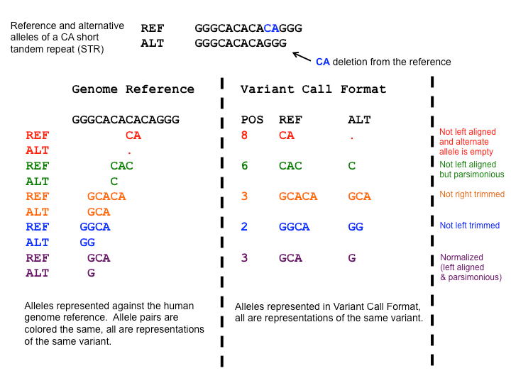  Open image in new tab
  
  

  .

A tool that can do this and also ensures that a VCF dataset conforms to standards in some other, less important respects is bcftools norm.

Hands-on: Post-processing FreeBayes calls

1. bcftools norm ( Galaxy version 1.15.1+galaxy3) with the following parameters:
   • “VCF/BCF Data”: the VCF output of FreeBayes tool
   • “Choose the source for the reference genome”: Use a built-in genome
     • “Reference genome”: Human: hg19 (or a similarly named option)

     Comment: Using the imported `hg19` sequence

     If you have imported the hg19 chr8 sequence as a fasta dataset into your history instead:

     • “Choose the source for the reference genome”: Use a genome from the history
       • “Reference genome”: your imported hg19 fasta dataset

   • “When any REF allele does not match the reference genome base”: ignore the problem (-w)
   • “Atomize”: No
   • “Left-align and normalize indels?”: Yes

   • “Perform deduplication for the folowing types of variant records”: do not deduplicate any records

     Freebayes is not producing any duplicate calls.

   • “~multiallelics”: split multiallelic sites into biallelic records (-)

     • “split the following variant types”: both

       We want to split both, multiallelic SNP and indel records.

   • “output_type”: uncompressed VCF

     We would like to keep the results human-readable. VCF is also what tools like SnpEff and GEMINI expect as input. Compressed, binary BCF is interesting for space-efficient long-term storage of large lists of variants.

You could try to look for the differences between the original and the normalized VCF dataset, but for convenience bcftools norm reports a brief summary of the actions it performed. Expand the dataset in the history (by clicking on its name) to see this output listing the total number of variant lines processed, along with the number of split, realigned and skipped records.

Variant annotation and reporting

A list of variants detected in a set of samples is a start, but to discover biologically or clinically relevant information in it is almost impossible without some additional tools and data. In particular, the variants in the list need to be:

• prioritized with respect to their potential relevance for the biological / clinical phenotype that is studied

  Even with exome sequencing, only a fraction of the detected variants will have a clear impact on the function of a protein (many variants will introduce silent mutations, or reside in intronic regions still covered by the exome-enriched sequencing data). Of these, many will have been observed before in healthy individuals arguing against them playing an important role in an adverse phenotype.

• filtered based on the inheritance pattern expected for a causative variant

  A multisample VCF file records the most likely genotypes of all samples at every variant site. Knowing which individuals (samples) are affected by a phenotype we can exclude variants with inheritance patterns that are incompatible with the observed inheritance of the phenotype.

• reported in a more human-friendly form

  While the VCF format can be used to encode all relevant information about any variant, it is hard for humans to parse that information.

  Ideally, one would like to generate simpler reports for any set of filtered and prioritized variants.

Get data

Our workhorse for annotating and reporting variants and the genes affected by them will be the GEMINI framework. GEMINI comes bundled with a wealth of annotation data for human variants from many different sources. These can be used to annotate any list of human variants conveniently, without the need for separate downloads and conversion between different annotation data formats.

Details: Custom annotations and GEMINI

Beyond its bundled annotation data, GEMINI also provides (limited) support for using custom annotations. The Somatic variant calling tutorial demonstrates the use of GEMINI annotate tool for this purpose.

The only additional annotation tool we need, for the purpose of this tutorial, is the tool SnpEff, which can annotate variants with their calculated effects on known genomic features. Because SnpEff is a generic tool that can be used on variants found in the genome of any organism we need to provide it with a so-called SnpEff genome file that holds the annotated features (genes, transcripts, translated regions, etc.) for our genome of interest.

While annotated variants are all we need to prioritize them as described above, filtering based on inheritance patterns requires a way to inform GEMINI about the relationship between our samples and their observed phenotypes. This is done through a so-called pedigree file in PED format, which is rather simple to generate manually.

Hands-on: Obtain SnpEff genome and GEMINI pedigree files

1. Download SnpEff functional genomic annotations

   Comment: Shortcut

   You can skip this step if the Galaxy server you are working on offers Homo sapiens: hg19 as a locally installed snpEff database. You can check the Genome source select list of the SnpEff eff ( Galaxy version 4.3+T.galaxy2) tool to see if this is the case.

   Use SnpEff Download ( Galaxy version 4.3+T.galaxy2) to download genome annotation database hg19.

2. Create a PED-formatted pedigree dataset describing our single-family sample trio:

   #family_id    name     paternal_id    maternal_id    sex    phenotype
   FAM           father   0              0              1      1
   FAM           mother   0              0              2      1
   FAM           proband  father         mother         1      2
   

   and set its datatype to tabular.

   Tip: Creating a new file

   • Click galaxy-upload Upload Data at the top of the tool panel
   • Select galaxy-wf-edit Paste/Fetch Data at the bottom
   • Paste the file contents into the text field
   • Change Type from “Auto-detect” to tabular* Press Start and Close the window

   Warning: Remember those sample names

   The above content of the pedigree dataset assumes you chose father, mother, proband as the sample names at the read mapping step (if you haven’t mapped the reads yourself, but started with the premapped data, you can safely skip this warning section). By now, these sample names will have been propagated through BWA-MEM and Freebayes to the VCF dataset of variants. It is important that you use matching sample names in the pedigree and in the VCF dataset, or GEMINI will not be able to connect the information in them.

   If you have chosen different sample names before, you have to adjust the pedigree dataset accordingly!

   Details: More on PED files

   The PED format is explained in the help section of GEMINI load ( Galaxy version 0.20.1+galaxy2).

   Take a moment and try to understand the information that is encoded in the PED dataset we are using here.

Variant annotation with functional genomic effects

We need to start annotating our variants with SnpEff simply because Gemini knows how to parse SnpEff-annotated VCFs, while GEMINI output cannot be used with SnpEff.

Hands-on: Adding annotations with SnpEff

1. SnpEff eff ( Galaxy version 4.3+T.galaxy2)
   • param-file “Sequence changes (SNPs, MNPs, InDels)”: the output of bcftools norm tool
   • “Input format”: VCF
   • “Output format”: VCF (only if input is VCF)
   • “Genome source”: Locally installed reference genome
     • “Genome”: Homo sapiens: hg19 (or a similarly named option)

     Comment: Using the imported `hg19` SnpEff genome database

     If you have imported the hg19 SnpEff genome database into your history instead:

     • “Genome source”: Downloaded snpEff database in your history
       • param-file “SnpEff4.3 Genome Data”: your imported hg19 SnpEff dataset.

   • “Produce Summary Stats”: Yes

Running the above job will produce two datasets. One is a Summary Stats HTML report, which contains some interesting general metrics such as a distribution of variants across gene features. The other one is the main annotation result - a VCF like the input, but with annotations of variant effects added to the INFO column.

Hands-on: Optional hands-on: Inspect the Summary Stats output produced by SnpEff

1. Display the dataset:
   • Click the galaxy-eye icon next to the HTML dataset generated by SnpEff to display its contents.

   Question

   One section in the report is Number of effects by type and region. Given that you are analyzing exome data, what is the most surprising aspect in this section? Do you have an idea how to explain it?

   Solution

   According to the report, intronic variants make up 50% of all variants detected!

   Exome capture kits are designed to capture exons plus a bit of surrounding sequence to ensure proper coverage of the exon ends including splice junction sites.

   Thus, even though intronic sequences are underrepresented in exome sequencing data, not all of them are eliminated. Since mutations in most intron bases are neutral, they can accumulate at higher frequency than most mutations in exons and, thus, still represent a relevant fraction of all detected variants.

Generating a GEMINI database of variants for further annotation and efficient variant queries

Next, we are going to use the SnpEff-annotated VCF as the basis for more exhaustive annotation with GEMINI. Unlike SnpEff, GEMINI does not just add annotations to a list of variants in VCF format. Instead the framework extracts the variants from the VCF input and stores them, together with newly added annotations, in an SQL database. It then lets you formulate queries for retrieving and reporting subsets of variants. The combined variant extraction/annotation/storage step is performed by the GEMINI load tool. In addition, that same tool can be used to incorporate sample pedigree info into the database.

Hands-on: Creating a GEMINI database from a variants dataset

1. GEMINI load ( Galaxy version 0.20.1+galaxy2) with
   • param-file “VCF dataset to be loaded in the GEMINI database”: the output of SnpEff eff tool
   • “The variants in this input are”: annotated with snpEff

   • “This input comes with genotype calls for its samples”: Yes

     Sample genotypes were called by Freebayes for us.

   • “Choose a gemini annotation source”: select the latest available annotations snapshot (most likely, there will be only one)
   • “Sample and family information in PED format”: the pedigree file prepared above
   • “Load the following optional content into the database”
     • param-check “GERP scores”
     • param-check “CADD scores”
     • param-check “Gene tables”
     • param-check “Sample genotypes”
     • param-check “variant INFO field”

     Leave unchecked the following:

     • “Genotype likelihoods (sample PLs)”

       Freebayes does not generate these values

     • “only variants that passed all filters”

       This setting is irrelevant for our input because Freebayes did not apply any variant filters.

Running this job generates a GEMINI-specific database dataset, which can only be processed with other GEMINI tools. The benefit, however, is that we now have variants, rich annotations and pedigree info stored in a format that enables flexible and highly efficient queries, which will greatly simplify our actual task to identify the variant responsible for the child’s disease!

Details: The GEMINI suite of tools

For a beginner, the sheer number of GEMINI tools may be a bit daunting and give the impression that this framework adds a lot of complexity. In practice, however, you will likely only need a very limited number of these tools for any given analysis. To help you get an overview, here is a list of the most general-purpose tools and their function:

• Every analysis will always start with GEMINI load tool to build the GEMINI database from a variant list in VCF format and the default annotations bundled with GEMINI.
• GEMINI amend tool and GEMINI annotate tool let you add additional information to a GEMINI database after it has been created. Use GEMINI amend to overwrite the pedigree info in a database with the one found in a given PED input, and GEMINI annotate to add custom annotations based on a VCF or BED dataset.
• GEMINI database info tool lets you peek into the content of a GEMINI database to explore, e.g, what annotations are stored in it.
• GEMINI query tool and GEMINI gene-wise tool are the two generic and most flexible tools for querying, filtering and reporting variants in a database. There is hardly anything you cannot do with these tools, but you need to know or learn at least some SQL-like syntax to use them.
• GEMINI inheritance pattern tool simplifies variant queries based on their inheritance pattern. While you could use the query and gene-wise tools for the same purpose, this tool allows you to perform a range of standard queries without typing any SQL. This tool is what we are going to use here to identify the causative variant.
• The remaining tools serve more specialized purposes, which are beyond the scope of this tutorial.

The Somatic variant calling tutorial demonstrates the use of the GEMINI annotate and GEMINI query tools, and tries to introduce some essential bits of GEMINI’s SQL-like syntax.

For a thorough explanation of all tools and functionality you should consult the GEMINI documentation.

Candidate variant detection

Let us now try to identify variants that have the potential to explain the boy child’s osteopetrosis phenotype. Remember that the parents are consanguineous, but both of them do not suffer from the disease. This information allows us to make some assumptions about the inheritance pattern of the causative variant.

Question

Which inheritance patterns are in line with the phenotypic observations for the family trio?

Hint: GEMINI easily lets you search for variants fitting any of the following inheritance patterns:

• Autosomal recessive
• Autosomal dominant
• X-linked recessive
• X-linked dominant
• Autosomal de-novo
• X-linked de-novo
• Compound heterozygous
• Loss of heterozygosity (LOH) events

Think about which of these might apply to the causative variant.

Solution

• Since both parents are unaffected the variant cannot be dominant and inherited.
• A de-novo acquisition of a dominant (or an X-linked recessive) mutation is, of course, possible.
• A recessive variant is a possibility, and a more likely one given the parents’ consanguinity.
• For both the de-novo and the inherited recessive case, the variant could reside on an autosome or on the X chromosome. Given that we provided you with only the subset of sequencing reads mapping to chr8, an X-linked variant would not be exactly instructive though ;)
• A compound heterozygous combination of variant alleles affecting the same gene is possible, but less likely given the consanguinity of the parents (as this would require two deleterious variant alleles in the gene circulating in the same family).
• A loss of heterozygosity (LOH) turning a heterozygous recessive variant into a homozygous one could be caused by uniparental disomy or by an LOH event early in embryonic development, but both these possibilities have an exceedingly small probability.

Based on these considerations it makes sense to start looking for inherited autosomal recessive variants first. Then, if there is no convincing candidate mutation among them, you could extend the search to de-novo variants, compund heterozygous variant pairs and LOH events - probably in that order.

Since our GEMINI database holds the variant and genotype calls for the family trio and the relationship between the family members, we can make use of GEMINI inheritance pattern tool to report all variants fitting any specific inheritance model with ease.

Below is how you can perform the query for inherited autosomal recessive variants. Feel free to run analogous queries for other types of variants that you think could plausibly be causative for the child’s disease.

Hands-on: Finding and reporting plausible causative variants

1. GEMINI inheritance pattern ( Galaxy version 0.20.1)
   • “GEMINI database”: the GEMINI database of annotated variants; output of GEMINI load tool
   • “Your assumption about the inheritance pattern of the phenotype of interest”: Autosomal recessive
     • param-repeat “Additional constraints on variants”

       • “Additional constraints expressed in SQL syntax”: impact_severity != 'LOW'

         This is a simple way to prioritize variants based on their functional genomic impact. Variants with low impact severity would be those with no obvious impact on protein function (i.e., silent mutations and variants outside coding regions)

     • “Include hits with less convincing inheritance patterns”: No

       This option is only meaningful with larger family trees to account for errors in phenotype assessment.

     • “Report candidates shared by unaffected samples”: No

       This option is only meaningful with larger family trees to account for alleles with partial phenotypic penetrance.

   • “Family-wise criteria for variant selection”: keep default settings

     This section is not useful when you have data from just one family.

   • In “Output - included information”
     • “Set of columns to include in the variant report table”: Custom (report user-specified columns)
       • “Choose columns to include in the report”:
         • param-check “alternative allele frequency (max_aaf_all)”
       • “Additional columns (comma-separated)”: chrom, start, ref, alt, impact, gene, clinvar_sig, clinvar_disease_name, clinvar_gene_phenotype, rs_ids

   Comment: Variant- vs gene-centric ClinVar information

   Most annotation data offered by GEMINI is variant-centric, i.e., annotations reported for a variant are specific to this exact variant. A few annotation sources, however, also provide gene-centric information, which applies to the gene affected by a variant, not necessarily the variant itself.

   In the case of ClinVar, the annotation fields/columns clinvar_sig and clinvar_disease_name refer to the particular variant, but clinvar_gene_phenotype provides information about the affected gene.

   Including the gene phenotype in the report can be crucial because a gene may be well known to be disease-relevant, while a particular variant may not have been clinically observed or been reported before.

Question

From the GEMINI reports you generated, can you identify the most likely candidate variant responsible for the child’s disease?

Details: More GEMINI usage examples

While only demonstrating command line use of GEMINI, the following tutorial slides may give you additional ideas for variant queries and filters:

• Introduction to GEMINI
• Identifying de novo mutations with GEMINI
• Identifying recessive gene candidates with GEMINI
• Identifying dominant gene candidates with GEMINI

Conclusion

It was not hard to find the most likely causative mutation for the child’s disease (you did find it, right?).

Even though it will not always provide as strong support for just one specific causative variant, analysis of whole-exome sequencing data of family trios (or other related samples) can often narrow down the search for the cause of a genetic disease to just a very small, manageable set of candidate variants, the relevance of which can then be addressed through standard methods.

Key points

• Exome sequencing is an efficient way to identify disease-relevant genetic variants.

• Freebayes is a good variant and genotype caller for the joint analysis of multiple samples. It is straightforward to use and requires only minimal processing of mapped reads.

• Variant annotation and being able to exploit genotype information across family members is key to identifying candidate disease variants. SnpEff and GEMINI, in particular, are powerful tools offered by Galaxy for that purpose.

Frequently Asked Questions

Useful literature

Further information, including links to documentation and original publications, regarding the tools, analysis techniques and the interpretation of results described in this tutorial can be found here.

Feedback

Did you use this material as an instructor? Feel free to give us feedback on how it went.
Did you use this material as a learner or student? Click the form below to leave feedback.

Citing this Tutorial

1. Wolfgang Maier, Bérénice Batut, Torsten Houwaart, Anika Erxleben, Björn Grüning, Exome sequencing data analysis for diagnosing a genetic disease (Galaxy Training Materials). https://training.galaxyproject.org/training-material/topics/variant-analysis/tutorials/exome-seq/tutorial.html Online; accessed TODAY
2. Hiltemann, Saskia, Rasche, Helena et al., 2023 Galaxy Training: A Powerful Framework for Teaching! PLOS Computational Biology 10.1371/journal.pcbi.1010752
3. Batut et al., 2018 Community-Driven Data Analysis Training for Biology Cell Systems 10.1016/j.cels.2018.05.012

BibTeX

@misc{variant-analysis-exome-seq,
author = "Wolfgang Maier and Bérénice Batut and Torsten Houwaart and Anika Erxleben and Björn Grüning",
	title = "Exome sequencing data analysis for diagnosing a genetic disease (Galaxy Training Materials)",
	year = "",
	month = "",
	day = ""
	url = "\url{https://training.galaxyproject.org/training-material/topics/variant-analysis/tutorials/exome-seq/tutorial.html}",
	note = "[Online; accessed TODAY]"
}
@article{Hiltemann_2023,
	doi = {10.1371/journal.pcbi.1010752},
	url = {https://doi.org/10.1371%2Fjournal.pcbi.1010752},
	year = 2023,
	month = {jan},
	publisher = {Public Library of Science ({PLoS})},
	volume = {19},
	number = {1},
	pages = {e1010752},
	author = {Saskia Hiltemann and Helena Rasche and Simon Gladman and Hans-Rudolf Hotz and Delphine Larivi{\`{e}}re and Daniel Blankenberg and Pratik D. Jagtap and Thomas Wollmann and Anthony Bretaudeau and Nadia Gou{\'{e}} and Timothy J. Griffin and Coline Royaux and Yvan Le Bras and Subina Mehta and Anna Syme and Frederik Coppens and Bert Droesbeke and Nicola Soranzo and Wendi Bacon and Fotis Psomopoulos and Crist{\'{o}}bal Gallardo-Alba and John Davis and Melanie Christine Föll and Matthias Fahrner and Maria A. Doyle and Beatriz Serrano-Solano and Anne Claire Fouilloux and Peter van Heusden and Wolfgang Maier and Dave Clements and Florian Heyl and Björn Grüning and B{\'{e}}r{\'{e}}nice Batut and},
	editor = {Francis Ouellette},
	title = {Galaxy Training: A powerful framework for teaching!},
	journal = {PLoS Comput Biol} Computational Biology}
}

                   

Galaxy Administrators: Install the missing tools

You can use Ephemeris's shed-tools install command to install the tools used in this tutorial.

shed-tools install [-g GALAXY] [-a API_KEY] -t <(curl https://training.galaxyproject.org/training-material/api/topics/variant-analysis/tutorials/exome-seq/tutorial.json | jq .admin_install_yaml -r)

Alternatively you can copy and paste the following YAML

---
install_tool_dependencies: true
install_repository_dependencies: true
install_resolver_dependencies: true
tools:
- name: bwa
  owner: devteam
  revisions: e188dc7a68e6
  tool_panel_section_label: Mapping
  tool_shed_url: https://toolshed.g2.bx.psu.edu/
- name: fastqc
  owner: devteam
  revisions: 5ec9f6bceaee
  tool_panel_section_label: FASTA/FASTQ
  tool_shed_url: https://toolshed.g2.bx.psu.edu/
- name: freebayes
  owner: devteam
  revisions: a5937157062f
  tool_panel_section_label: Variant Calling
  tool_shed_url: https://toolshed.g2.bx.psu.edu/
- name: samtools_rmdup
  owner: devteam
  revisions: 586f9e1cdb2b
  tool_panel_section_label: SAM/BAM
  tool_shed_url: https://toolshed.g2.bx.psu.edu/
- name: bcftools_norm
  owner: iuc
  revisions: ebb2e12a6de1
  tool_panel_section_label: Variant Calling
  tool_shed_url: https://toolshed.g2.bx.psu.edu/
- name: gemini_inheritance
  owner: iuc
  revisions: 2c68e29c3527
  tool_panel_section_label: Gemini
  tool_shed_url: https://toolshed.g2.bx.psu.edu/
- name: gemini_load
  owner: iuc
  revisions: 2270a8b83c12
  tool_panel_section_label: Gemini
  tool_shed_url: https://toolshed.g2.bx.psu.edu/
- name: multiqc
  owner: iuc
  revisions: abfd8a6544d7
  tool_panel_section_label: Quality Control
  tool_shed_url: https://toolshed.g2.bx.psu.edu/
- name: samtools_view
  owner: iuc
  revisions: 5826298f6a73
  tool_panel_section_label: SAM/BAM
  tool_shed_url: https://toolshed.g2.bx.psu.edu/
- name: snpeff
  owner: iuc
  revisions: 9473cd297a76
  tool_panel_section_label: Variant Calling
  tool_shed_url: https://toolshed.g2.bx.psu.edu/
- name: snpeff
  owner: iuc
  revisions: 9473cd297a76
  tool_panel_section_label: Variant Calling
  tool_shed_url: https://toolshed.g2.bx.psu.edu/
- name: trimmomatic
  owner: pjbriggs
  revisions: d94aff5ee623
  tool_panel_section_label: FASTA/FASTQ
  tool_shed_url: https://toolshed.g2.bx.psu.edu/

Feedback

5 stars	19
4 stars	2
3 stars	4
1 stars	3

March 2024

• 5 stars: Liked: Instructions were very clear

May 2023

• 3 stars: Disliked: Gemini is no longer used

April 2023

• 5 stars: Liked: Most part of the instructions were very clear and detailed. Disliked: There are still some part of the tutorial which can be a little more clear, for example at "Hands-on: Generating FreeBayes calls" I was confused and took a while to figure out.

March 2023

• 3 stars: Disliked: You should specify that you can't feed GEMINI tool more recent versions of hg19 at the outset. I used a more recent version hg38 throughout my analysis, only to get to the last step and realize that I had to start over using hg19. Also, GEMINI is not available on usegalaxy.org, only on galaxy.eu, and I am having a lot of difficulty importing my datasets over since the tags for my PED file disappear on transfer. Extremely frustrating end result for what I originally thought was a great tutorial!

November 2022

• 4 stars: Liked: detailed explanation of variant calling and genotype calling
• 3 stars: Liked: This tutorial gives a comprehensive overview about all analysis steps and important parameters involved. Disliked: Where is the actual hands-on command code, which is generated after all parameter boxes have been checked, and the 'submit button' is clicked? Where are the actual tool commands for each step, a user would need to perform these analysis steps on the command line? I know these can be displayed in Galaxy, but it would be helpful to show them in the tutorials as well.

March 2022

• 5 stars: Liked: The step-by-step approach and the additional explanations for some input fields Disliked: Perhaps an additional indication of which patch of the hg19 is recognised as the database of the SNPeff eff output of GEMINI load. It took me several attempts to realise that it must be the unpatched version.

November 2021

• 3 stars: Liked: Nice features and understandable handling for beginners Disliked: Some data and tools are not at the described places; specifically genome annotation fasta and snpTools... snpEff is not existing, so I used snpEff eff; snpSift Annotate exists twice with different features. Description on how to create the pedigree file.

June 2021

• 5 stars: Liked: Oustanding material! Disliked: Nothing!

May 2021

• 5 stars: Liked: all of it Disliked: nothing - it's perfect
• 5 stars: Liked: Gareth, Melissa and Khalid (I was in breakout room 3) were all incredibly helpful and it went at a good pace. It was VERY helpful getting the course material ahead of the workshop, which allowed time to familiarise myself with the content. Disliked: I think it was on the mark for me.

March 2021

• 5 stars: Liked: Going to use this in Australia soon (late May 2021)- excited about it. More feedback to come afterwards no doubt! Disliked: I can see in the intro that this tutorial is set up for raw (fastq) and BAM data entry points. This is great but I was hoping you could include a workflow for fastq to BAM. I realise it is in the full workflow so I took the liberty of comparing the two offered workflows and trimmed down to a QC to BAM workflow (https://usegalaxy.org.au/u/gareth-qfab/w/copy-of-exome-seq-training-full-w-cached-ref-imported-from-uploaded-file ). I understand we can do this elsewhere but good to have it consistent within this tutorial. Tested on Zenodo data and works fine. Thanks, Gareth

February 2021

• 5 stars: Liked: Concentration on the essential aspects with the possibility to further deepen the knowledge about the individual tools

June 2020

• 4 stars: Liked: I liked that it was very specific and went step by step on how to do everything. nothing was left out. Disliked: I would like to know how to take the vcf file and identify polymorphic sites in all three individuals.

March 2020

• 5 stars: Liked: Clear, stepwise Disliked: Gemini load dialog in usegalaxy.eu suggested the SnpEff eff output file was 'unavailable' to use. It made me go back and check things before pressing on regardless. Not a problem with the tutorial per se. Thanks
• 5 stars: Liked: Very accessible, especially if you compare the galaxy ui to something like bash. Disliked: -

July 2019

• 5 stars: Liked: Even simple steps were explained.
• 5 stars: Liked: looking at genes

December 2018

• 1 stars: Disliked: unfortunately in compare with others tutorial, this is very unclear and o'm not satisfied please improve this very important tutorial with clear and accurate dive.

November 2018

• 1 stars: Liked: I like the idea of it Disliked: It seems impossible to complete. The training data is not available in the shared data link. If it is, it's too hard to find. A more general point would be to explain how the tutorial could be used on other data sets. or ref genomes. For this I tried using an hg19 fasta file from another data set, but got an error about indexing. So I guess, explaining how the training data sets are pre-formatted would help when trying to use sets from other sources