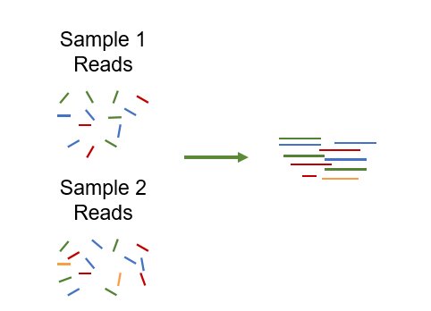
Metagenomics involves the extraction, sequencing and analysis of combined genomic DNA from entire microbiome samples. It includes then DNA from many different organisms, with different taxonomic background.
Reconstructing the genomes of microorganisms in the sampled communities is critical step in analyzing metagenomic data. To do that, we can use assembly and assemblers, i.e. computational programs that stich together the small fragments of sequenced DNA produced by sequencing instruments.
Assembling seems intuitively similar to putting together a jigsaw puzzle. Essentially, it looks for reads “that work together” or more precisely, reads that overlap. Tasks like this are not straightforward, but rather complex because of the complexity of the genomics (specially the repeats), the missing pieces and the errors introduced during sequencing.
Comment
Do you want to learn more about the principles behind single genome assembly? Follow our tutorials.
Metagenomic assembly is further complicated by
the large volume of data produced
the quality of the sequence
the unequal representation of members of the microbial community
the presence of closely related microorganisms with similar genomes
the presence of several strains of the same microorganism
an insufficient amount of data for minor community members
For assembly, there are 3 main strategies:
Greedy extension
Overlap Layout Consensus
De Bruijn graphs. The following figure illustrates these strategies in brief.
The nice paper Miller et al. 2010 on assemblers based on these algorithms will help you to better understand how they work.
For metagenomic assembly, several tools exist: metaSPAdes (Nurk et al. 2017), MEGAHIT (Li et al. 2015), etc. The different assemblers have different computational characteristics and their performance varies according to the microbiome as shown in by both rounds of Critical Assessment of Metagenome Interpretation initiative (Sczyrba et al. 2017, Meyer et al. 2022, Meyer et al. 2021). The preference of one assembler over another depends on the purpose at hand.
In this tutorial, we will learn how to run metagenomic assembly tool and evaluate the quality of the generated assemblies. To do that, we will use data from the study: Temporal shotgun metagenomic dissection of the coffee fermentation ecosystem. For an in-depth analysis of the structure and functions of the coffee microbiome, a temporal shotgun metagenomic study (six time points) was performed. The six samples have been sequenced with Illumina MiSeq utilizing whole genome sequencing.
Based on the 6 original dataset of the coffee fermentation system, we generated mock datasets for this tutorial.
Figure 4: Individual assembly followed by de-replication vs co-assembly. Source: dRep documentation
Co-assembly is more commonly used than individual assembly and then de-replication after binning. But in this tutorial, to show all steps, we will run an individual assembly.
Comment
Sometimes it is important to run assembly tools both on individual samples and on all pooled samples, and use both outputs to get the better outputs for the certain dataset.
As mentioned in the introduction, several tools are available for metagenomic assembly. But 2 are the most used ones:
MetaSPAdes (Nurk et al. 2017): an short-read assembler designed specifically for large and complex metagenomics datasets
MetaSPAdes is part of the SPAdes toolkit, which has several assembly pipelines. Since SPAdes handles non-uniform coverage, it is useful for assembling simple communities, but metaSPAdes also handles other problems, allowing it to assemble complex communities’ metagenomes.
As input for metaSPAdes it can accept short reads. However, there is an option to use additionally long reads besides short reads to produce hybrid input.
MEGAHIT (Li et al. 2015): a single node assembler for large and complex metagenomics NGS reads, such as soil
It makes use of succinct de Bruijn graph (SdBG) to achieve low memory assembly.
Both tools are available in Galaxy. But currently, only MEGAHIT can be used in individual mode for several samples.
Hands-on: Individual assembly of short-reads with MEGAHIT
MEGAHIT ( Galaxy version 1.2.9+galaxy0) with parameters:
“Select your input option”: Paired-end collection
“Run in batch mode?”: Run individually
Comment
To run as co-assembly, select Merge all fastq pair-end, instead of Run individually
param-collection“Select a paired collection”: Raw reads
In Basic assembly options
“K-mer specification method”: Specify min, max, and step values
“Minimum kmer size”: 21
“Maximum kmer size”: 91
“Increment of kmer size of each iteration”: 12
MEGAHIT produced a collection of output assemblies - one per sample - that can be proceeded further in binning step and then de-replication. The output contains contigs, contiguous lengths of genomic sequences in which bases are known to a high degree of certainty.
Contrary to MetaSPAdes, MEGAHIT does not output scaffolds, i.e. segments of genome sequence reconstructed fron contigs and gaps. The gaps occur when reads from the two sequenced ends of at least one fragment overlap with other reads from two different contigs (as long as the arrangement is otherwise consistent with the contigs being adjacent). It is possible to estimate the number of bases between contigs based on fragment lengths.
Comment
Since the assembly process would take ~1h we are just going to import the results of the assembly previously run.
Hands-on: Import generated assembly files
Import the six contig files from Zenodo or the Shared Data library:
Quast main output are HTML reports which aggregate different metrics.
Assembly statistics
On the top of each report is a table with in rows statistics for contigs larger than 500 bp for the different sample assemblies (columns). Let’s now look at the table and go from top to bottom:
Genome statistics
Genome fraction (%): percentage of aligned bases in the reference genome
A base in the reference genome is counted as aligned if at least one contig has at least one alignment to this base.
We did not provide any reference there, but metaQuast try to identify genome content of the metagenome by aligning contigs to SILVA 16S rRNA database. For each assembly, 50 reference genomes with top scores are chosen. The full reference genomes of the identified organisms are afterwards downloaded from NCBI to map the assemblies on them and compute the genome fractions.
For each identified genomes, the genome fraction is given when clicking on Genome fraction (%)
Question
What is the genome fraction for ERR2231568? And for ERR2231572?
Which reference genome has the highest genome fraction for ERR2231568? And for ERR2231572?
The genome fraction is 30.22% for ERR2231568 and 58.73% for ERR2231572
The highest genome fraction was found for Leuconostoc pseudomesenteroides for ERR2231568 (844%) and for Lactobacillus for ERR2231572 (91%). The genomes of Leuconostoc pseudomesenteroides and Lactobacillus could be then almost completely recovered from the assemblies of ERR2231568 and ERR2231572 respectively.
Duplication ratio: total number of aligned bases / genome fraction * reference length
If an assembly contains many contigs that cover the same regions of the reference, the duplication ratio may be much larger than 1.
Question
What is the duplication ratio for ERR2231568? And for ERR2231572?
Which reference genome has the highest duplication ratio for ERR2231568? And for ERR2231572?
The duplication ratio is 1.068 for ERR2231568 and 1.1 for ERR2231572 (column ERR2231572 in ERR2231572 report)
The highest duplication ratio was found for Gluconobacter kondonii for ERR2231568 (1.156) and for Lactobacillus brevis KB290 for ERR2231572 (1.178).
Read mapping: results of the mapping of the raw reads on the different assemblies (only if the “Reads options” is not disabled)
Question
What is the % of read mapped for ERR2231568 assembly to ERR2231568 raw reads? And for ERR2231572 assembly to ERR2231572 raw reads?
What is the percentage of reads used to build the assemblies for ERR2231568? and ERR2231572?
79.47% of ERR2231568 raw reads were mapped to ERR2231568 assembly and 86.98% of ERR2231572 raw reads to ERR2231572 assembly.
79.47% of reads were used to the assemblies for ERR2231568 and 86.97% for ERR2231572.
“Save the Bowtie2 mapping statistics to the history”: Yes
Inspect the mapping statistics output
Question
What is the overall alignment rate for ERR2231567? and ERR2231571?
What is the percentage of reads used in assemblies for ERR2231567? and ERR2231571?
The overall alignment rate for ERR2231567 is 65.97% and 73.67% for ERR2231571
65.97% of the reads were used in assemblies for ERR2231567 and 73.67% for ERR2231571.
Misassemblies: joining sequences that should not be adjacent.
Quast identifies missassemblies by mapping the contigs to the reference genomes of the identified organisms. 3 types of misassemblies can be identified:
How many relocations has been found for ERR2231568? And for ERR2231572?
For which reference genomes are there the most relocation found for ERR2231568? And for ERR2231572?
78 for ERR2231568 and 151 for ERR2231572
Leuconostoc pseudomesenteroides and Tatumella morbirosei for ERR2231568 and Lactobacillus plantarum argentoratensis for ERR2231572
Translocation occur when a contig has mapped on more than one reference chromosomes
Question
How many translocations has been found for ERR2231568? And for ERR2231572?
For which reference genomes are there the most translocations found for ERR2231568? And for ERR2231572?
What are the interspecies translocations?
How many interspecies translocations has been found for ERR2231568? And for ERR2231572?
25 for ERR2231568 and 55 for ERR2231572.
Leuconostoc pseudomesenteroides for ERR2231568 and Lactobacillus vaccinostercus for ERR2231572.
Interspecies translocations are translocations where a contig has mapped on different reference genomes.
80 for ERR2231568 and 144 for ERR2231572.
Inversion occurs when a contig has two consecutive mappings on the same chromosome but in different strands
Question
How many inversion has been found for ERR2231568? And for ERR2231572?
For which reference genomes are there the most inversions found for ERR2231568? And for ERR2231572?
4 for ERR2231568 and 6 for ERR2231572.
Tatumella morbirosei for ERR2231568 and Lactobacillus sp for ERR2231572.
Mismatches or mismatched bases in the contig-reference alignment
Question
How many mismatches have been identified for ERR2231568? And for ERR2231572?
For which reference genomes are there the most mismatches for ERR2231568? And for ERR2231572?
503,352 for ERR2231568 and 287,270 for ERR2231572.
Pantoea rwandensis for ERR2231568 and Leuconostoc brevis KB290 for ERR2231572.
Statistics without reference
# contigs: total number of contigs
Question
How many contigs are for ERR2231568? And for ERR2231572?
How many sequences are in the output of MEGAHIT for ERR2231568? And for ERR2231572?
Why are these numbers different from the number of sequences in the output of MEGAHIT?
Which statistics in the metaQUAST report corresponds to number of sequences in the output of MEGAHIT?
Which reference genomes have the most contigs (\(\geq\) 500 bp) in ERR2231568? And in ERR2231572?
66,434 contigs for ERR2231568 and 36,112 for ERR2231572.
In the outputs of MEGAHIT, there are 228,719 contigs for ERR2231568 and 122,526 contigs.
The numbers are lower in the metaQUAST results because metaQUAST reports there only the contigs longer than 500bp.
The # contigs (>= 0 bp)
Except the non aligned contigs, Tatumella morbirosei for ERR2231568 and Leuconostoc brevis KB290 for ERR2231572.
Largest contig: length of the longest contig in the assembly
Question
What is the length of the longest contig in ERR2231568? And in ERR2231572?
Is the longest contig assigned to a reference genome in ERR2231568? And in ERR2231572?
63,871 bp in ERR2231568 and 65,608 for ERR2231572.
It is assigned to Leuconostoc pseudomesenteroides KCTC 3652 in ERR2231568 and not assigned in ERR2231572.
N50: length for which the collection of all contigs of that length or longer covers at least half an assembly
N50 statistic defines assembly quality in terms of contiguity. If all contigs in an assembly are ordered by length, the N50 is the minimum length of contigs that contains 50% of the assembled bases. For example, an N50 of 10,000 bp means that 50% of the assembled bases are contained in contigs of at least 10,000 bp.
Another example. Let’s consider 9 contigs with the lengths 2, 3, 4, 5, 6, 7, 8, 9, and 10:
The sum of the length is 54
Half of the sum is 27
10 + 9 + 8 = 27 (half the length of the sequence)
N50 = 8, i.e. the size of the contig which, along with the larger contigs, contain half of sequence of a particular genome
Question
What is N50 for ERR2231568? And for ERR2231572?
What is N90?
921 for ERR2231568 and 1,233 for ERR2231572.
N90 is similar to the N50 metric but with 90% of of the sum of the lengths of all contigs
When comparing N50 values from different assemblies, the assembly sizes must be the same size in order for N50 to be meaningful.
Also the N50 alone is not a useful measure to assess the quality of an assembly. For example, the assemblies with the following contig lengths:
3, 3, 3, 3, 3, 3, 3, 3, 3, 3, 25, 25, 150, 1500
50, 500, 530, 650
Both assemblies have the same N50 although one is more contiguous than the other.
L50: number of contigs equal to or longer than N50
In other words, L50, for example, is the minimal number of contigs that cover half the assembly.
If we take the previous example in N50, L50 = 3.
Question
What is the L50 for ERR2231568? And for ERR2231572?
17,280 for ERR2231568 and 7,496 for ERR2231572.
Icarus contig browser
Icarus generates contig size viewer and one or more contig alignment viewers (if reference genome/genomes are provided) that are accessible from the HTML report, by clicking on View on Icarus contig browser.
Contig size viewer
This viewer draws contigs ordered from longest to shortest. Let’s inspect this viewer for ERR2231568.
Question
Open the Contig size viewer for ERR2231568 and define start as 0 and end as 500000
What is the color of the first contig? Why?
What is the red contig?
The first contig is white because >50% of the contigs is unaligned. By clicking on the contig, we see that only a small block is aligned: 223.41 – 223.65 kbp to Leuconostoc_pseudomesenteroides_KCTC_3652_NZ_BMBP01000002.1.
The red contig is a missamblied contig: it contains 2 blocks, with a translocation between them.
Click Main menu on the top left to go back to the main Icarus page.
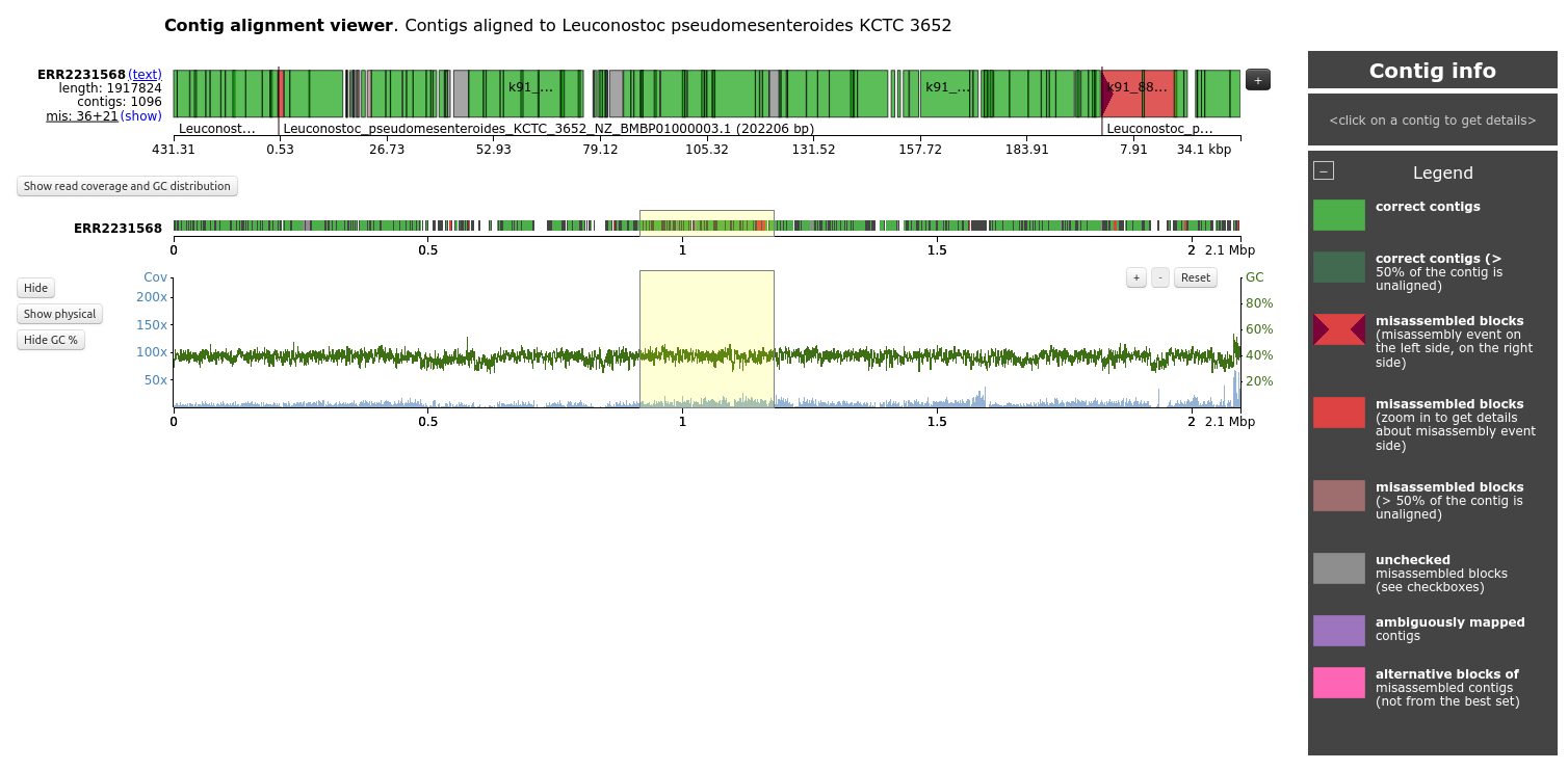
Contig alignment viewer
If a reference genome is provided, there should be a table on the main Icarus page that looks like:
Genome
# fragments
Length, bp
Mean genome fraction, %
# misassembled blocks
Gluconobacter oxydans H24
2
3 816 232
10.989
38
Kosakonia cowanii
5
4 806 998
28.224
60
Lactococcus lactis subsp. lactis CV56
6
2 518 737
18.940 23
When clicking on the genome name, the contigs are displayed according to their mapping to the reference genome. The viewer can additionally visualize genes, operons, and read coverage distribution along the genome, if any of those were fed to QUAST.
Question
Open the Contig alignment viewer for ERR2231568 and Leuconostoc pseudomesenteroides KCTC 3652, the most covered by contigs
How are the organized the contigs on the top?
What the different colors for the contigs?
Why is there a big red block on the right?
What is the graph on the bottom?
The contigs are displayed based on their mapping on the reference genome of Leuconostoc pseudomesenteroides KCTC 3652
The different colors represent the different status for the contig: correct contigs, correct contigs but with >50% of the contig unaligned, misassembled blocks. unchecked misassembled blocks, ambiguously mapped contigs, alternative blocks of misassembled contigs, etc.
The big red block on the right is contig k91_88833 with a misassembly on the left side, and overlap with 2 other contigs
The graph on the bottom represents the GC percentage and coverage by contigs along the reference genome
Current metagenome assemblers like MEGAHIT and MetaSPAdes use graphs, most typically a de Bruijn graph to stich reads together. In an ideal case, the graph would contain one distinct path for each genome of each micro-organisms, but complexities such as repeated sequences usually prevent this.
Assembly graphs contain then branching structures: one node may lead into multiple others. Contigs correspond to the longest sequences in the graph that can be determined unambiguously. They are the final results of most assembler. But the assembly graph contains more information. It can be useful for finding sections of the graph, such as rRNA, or to try to find parts of a genome.
Bandage (Wick et al. 2015) is a tool creating interactive visualisations of assembly graphs.
Hands-on: Visualization the assembly graph
megahit contig2fastg ( Galaxy version 1.1.3+galaxy10) with parameters:
param-collection“Contig file”: Output of MEGAHIT
“K-mer length”: 91
Comment
To get the value, you need to
Go into the MEGAHIT output collection
Expand one of the contig file by clicking on it in the history
Check in the dataset peek the name of the contig
Extract the value after the first k in the contig names
Bandage Image ( Galaxy version 0.8.1+galaxy4) with parameters:
param-collection“Graphical Fragment Assembly”: Output of megahit contig2fastg
The graph is quite disconnected. On the top, we can see the longer stretches, that includes multiples contigs (each contig having a different color). On the bottom are the shortest stretches or single contigs.
But it is really hard to read or extract any information from the graph. Let’s inspect the information about the assembly graph
Hands-on: Visualization the *de novo* assembly graph
Bandage Info ( Galaxy version 0.8.1+galaxy2) with parameters:
param-collection“Graphical Fragment Assembly”: Output of megahit contig2fastg
Column join ( Galaxy version 0.0.3) with parameters:
param-collection“Tabular files”: Output of Bandage Info
Inspect the generated output
Question
How many nodes are in the graph for ERR2231568? And for ERR2231572? What does they correspond to?
How many edges are in the graph for ERR2231568? And for ERR2231572? What is the impact of these numbers in relation to the number of nodes on the graph?
How many connected components are there for ERR2231568? And for ERR2231572? What does they correspond to?
What is the percentage of dead ends are there for ERR2231568? And for ERR2231572?
What are the smallest and larges edge overlaps?
What is the largest component? For which sample?
What is the shortest node? What does they correspond to?
There are 228,719 nodes for ERR2231568 and 122,526 for ERR2231572. They correspond to the number of contigs
There are 16,580 edges for ERR2231568 and 13,993 for ERR2231572. There are less edges than nodes in the graph. It means that many nodes/contigs are disconnected
There are 212,598 connected components, i.e. number of regions of the graph which are disconnected from each other, for ERR2231568 and 109,044 for ERR2231572
There are 94.0702% dead ends, i.e. the end of a node not connected to any other nodes, for ERR2231568 and 90.7032% for ERR2231572. It confirms the previous observation
The smallest and larges edge overlaps are 91bp, i.e. the k-mer length
The largest component is 340,003 bp for ERR2231567
The shortest node is 200 bp, i.e. the minimal size for a contig
Conclusion
Metagenomic data can be assembled to, ideally, obtain the genomes of the species that are represented within the input data. But metagenomic assembly is complex and there are
different approaches like de Bruijn graphs methods
different strategies, such as co-assembly, when we assembly all samples together, and individual assembly, when we assembly samples one by one
different tools like MetaSPAdes and MEGAHIT
Once the choices made, metagenomic assembly can start:
Input data are assembled to obtain contigs and sometimes scaffolds
Assembly quality is evaluated with various metrics
The assembly graph can be visualized.
Once all these steps done, we can move to the next phase to build Metagenomics Assembled Genomes (MAGs): binning
Kececioglu, J., and J. Ju, 2001 Separating repeats in DNA sequence assembly, pp. 176–183 inProceedings of the fifth annual international conference on Computational biology, RECOMB ’01, Association for Computing Machinery, New York, NY, USA. 10.1145/369133.369192
Miller, J. R., S. Koren, and G. Sutton, 2010 Assembly Algorithms for Next-Generation Sequencing Data. Genomics 95: 315–327. 10.1016/j.ygeno.2010.03.001
Gurevich, A., V. Saveliev, N. Vyahhi, and G. Tesler, 2013 QUAST: quality assessment tool for genome assemblies. Bioinformatics (Oxford, England) 29: 1072–1075. 10.1093/bioinformatics/btt086
Li, D., C.-M. Liu, R. Luo, K. Sadakane, and T.-W. Lam, 2015 MEGAHIT: an ultra-fast single-node solution for large and complex metagenomics assembly via succinct de Bruijn graph. Bioinformatics 31: 1674–1676. 10.1093/bioinformatics/btv033
Wick, R. R., M. B. Schultz, J. Zobel, and K. E. Holt, 2015 Bandage: interactive visualization of de novo genome assemblies. Bioinformatics 31: 3350–3352. 10.1093/bioinformatics/btv383
Mikheenko, A., V. Saveliev, and A. Gurevich, 2016 MetaQUAST: evaluation of metagenome assemblies. Bioinformatics (Oxford, England) 32: 1088–1090. 10.1093/bioinformatics/btv697
Nurk, S., D. Meleshko, A. Korobeynikov, and P. A. Pevzner, 2017 metaSPAdes: a new versatile metagenomic assembler. Genome Research 27: 824–834. Company: Cold Spring Harbor Laboratory Press Distributor: Cold Spring Harbor Laboratory Press Institution: Cold Spring Harbor Laboratory Press Label: Cold Spring Harbor Laboratory Press Publisher: Cold Spring Harbor Lab. 10.1101/gr.213959.116
Sczyrba, A., P. Hofmann, P. Belmann, D. Koslicki, S. Janssen et al., 2017 Critical Assessment of Metagenome Interpretation—a benchmark of metagenomics software. Nature Methods 14: 1063–1071. Number: 11 Publisher: Nature Publishing Group. 10.1038/nmeth.4458
Evans, J. T., and V. J. Denef, 2020 To Dereplicate or Not To Dereplicate? mSphere 5: e00971–19. Publisher: American Society for Microbiology. 10.1128/mSphere.00971-19
Meyer, F., T.-R. Lesker, D. Koslicki, A. Fritz, A. Gurevich et al., 2021 Tutorial: assessing metagenomics software with the CAMI benchmarking toolkit. Nature Protocols 16: 1785–1801. Number: 4 Publisher: Nature Publishing Group. 10.1038/s41596-020-00480-3
Meyer, F., A. Fritz, Z.-L. Deng, D. Koslicki, T. R. Lesker et al., 2022 Critical Assessment of Metagenome Interpretation: the second round of challenges. Nature Methods 19: 429–440. Number: 4 Publisher: Nature Publishing Group. 10.1038/s41592-022-01431-4
Feedback
Did you use this material as an instructor? Feel free to give us feedback on how it went.
Did you use this material as a learner or student? Click the form below to leave feedback.
Hiltemann, Saskia, Rasche, Helena et al., 2023 Galaxy Training: A Powerful Framework for Teaching! PLOS Computational Biology 10.1371/journal.pcbi.1010752
Batut et al., 2018 Community-Driven Data Analysis Training for Biology Cell Systems 10.1016/j.cels.2018.05.012
@misc{assembly-metagenomics-assembly,
author = "Polina Polunina and Bérénice Batut",
	title = "Assembly of metagenomic sequencing data (Galaxy Training Materials)",
	year = "",
	month = "",
	day = ""
	url = "\url{https://training.galaxyproject.org/training-material/topics/assembly/tutorials/metagenomics-assembly/tutorial.html}",
	note = "[Online; accessed TODAY]"
}
@article{Hiltemann_2023,
	doi = {10.1371/journal.pcbi.1010752},
	url = {https://doi.org/10.1371%2Fjournal.pcbi.1010752},
	year = 2023,
	month = {jan},
	publisher = {Public Library of Science ({PLoS})},
	volume = {19},
	number = {1},
	pages = {e1010752},
	author = {Saskia Hiltemann and Helena Rasche and Simon Gladman and Hans-Rudolf Hotz and Delphine Larivi{\`{e}}re and Daniel Blankenberg and Pratik D. Jagtap and Thomas Wollmann and Anthony Bretaudeau and Nadia Gou{\'{e}} and Timothy J. Griffin and Coline Royaux and Yvan Le Bras and Subina Mehta and Anna Syme and Frederik Coppens and Bert Droesbeke and Nicola Soranzo and Wendi Bacon and Fotis Psomopoulos and Crist{\'{o}}bal Gallardo-Alba and John Davis and Melanie Christine Föll and Matthias Fahrner and Maria A. Doyle and Beatriz Serrano-Solano and Anne Claire Fouilloux and Peter van Heusden and Wolfgang Maier and Dave Clements and Florian Heyl and Björn Grüning and B{\'{e}}r{\'{e}}nice Batut and},
	editor = {Francis Ouellette},
	title = {Galaxy Training: A powerful framework for teaching!},
	journal = {PLoS Comput Biol} Computational Biology}
}
Funding
These individuals or organisations provided funding support for the development of this resource
Questions:
Open image in new tab

 Open image in new tab
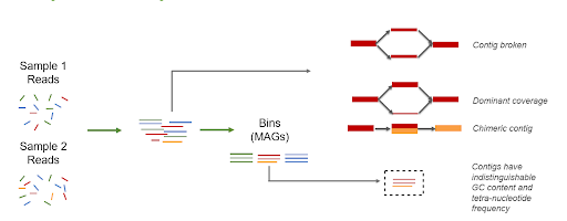 Open image in new tab
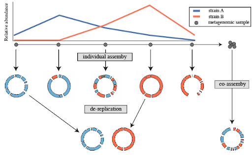 Open image in new tab
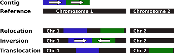 Open image in new tab
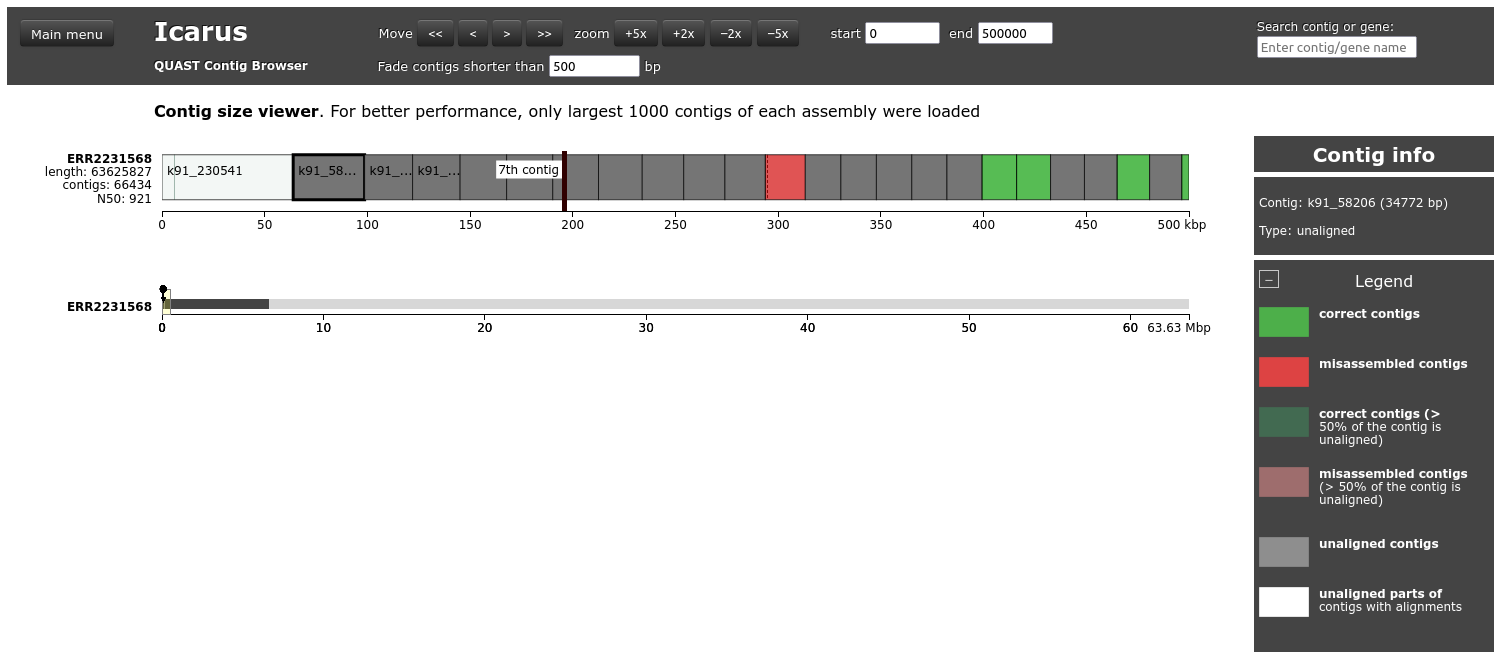
Open image in new tab